02_Vectors & Higher Dimension Motion

1. Kinematics in Higher Dimensions

This section contrasts 2D motion equations in standard versus rotated coordinate systems, followed by the generalized vector forms.

• Standard Coordinate System (Vertical \(y\)-axis):

  For a projectile launched horizontally with initial velocity \(v_0\) from \((x_0, y_0)\):

  \[ x = x_0 + v_0t \]
  \[ y = y_0 - \frac{1}{2}gt^2 \]

• Rotated Coordinate System:

  For axes tilted by an angle \(\theta\) relative to the standard horizontal/vertical:

  \[ x = x_0' + v_0 \cos\theta t - \frac{1}{2}\sin\theta g t^2 \]
  \[ y = y_0' - v_0 \sin\theta t - \frac{1}{2}g \cos\theta t^2 \]

• General Vector Form:

  Kinematic equations can be written completely independent of the coordinate system:

  \[ \vec{v} = \vec{v}_0 + \vec{a}t \]
  \[ \vec{r} = \vec{r}_0 + \vec{v}_0t + \frac{1}{2}\vec{a}t^2 \]

---

2. Vector Fundamentals

This section outlines the basic definitions, notations, and algebraic rules for vectors.

• Definition of Vector vs. Scalar:

  • Vector: Has direction, magnitude, and follows specific rules of addition.

  • Scalar: Has magnitude only (no direction).

• Vector Representation & Position (\(\vec{r}\)):

  Using basis vectors \(\vec{e}_i\):

  \[ \vec{r} = \{\vec{e}_1, \vec{e}_2\} \binom{x}{y} = x\vec{e}_1 + y\vec{e}_2 \]

  For general vectors in \(n\)-dimensions:

  \[ \vec{a} = \{\vec{e}_1, \dots, \vec{e}_n\} \begin{pmatrix} a_1 \\ \vdots \\ a_n \end{pmatrix}, \quad \vec{b} = \{\vec{e}_1, \dots, \vec{e}_n\} \begin{pmatrix} b_1 \\ \vdots \\ b_n \end{pmatrix} \]

• Basic Operations:

  • Vector Addition: \(\vec{a} + \vec{b} = \sum_i a_i\vec{e}_i + \sum_i b_i\vec{e}_i = \sum_i (a_i + b_i)\vec{e}_i\)

  • Commutative Law: \(\vec{a} + \vec{b} = \vec{b} + \vec{a}\)

  • Associative Law: \((\vec{a} + \vec{b}) + \vec{c} = \vec{a} + (\vec{b} + \vec{c})\)

  • Negative: \(\vec{a} + (-\vec{a}) = 0\)

  • Subtraction: \(\vec{a} - \vec{b} = \vec{a} + (-\vec{b})\)

  • Multiply by a Scalar (\(\alpha\)): \(\alpha\vec{a} = \alpha \left(\sum_i a_i\vec{e}_i\right) = \sum_i (\alpha a_i)\vec{e}_i\)

---

3. Scalar (Dot) Product

This section defines the dot product and how it behaves in Cartesian versus non-Cartesian spaces.

• General Definition:

  \[ \vec{a} \cdot \vec{b} = \left(\sum_i a_i\vec{e}_i\right) \cdot \left(\sum_j b_j\vec{e}_j\right) = \sum_i \sum_j a_i b_j (\vec{e}_i \cdot \vec{e}_j) \]

• Cartesian Coordinates:

  Basis vectors are orthogonal: \(\vec{e}_i \cdot \vec{e}_j = \delta_{ij}\) (Kronecker delta).

  This simplifies the scalar product to:

  \[ \Rightarrow \vec{a} \cdot \vec{b} = \sum_i a_i b_i = (a_1, \dots, a_n) \begin{pmatrix} b_1 \\ \vdots \\ b_n \end{pmatrix} \]

• Properties & Definitions:

  • Commutative Law: \(\vec{a} \cdot \vec{b} = \vec{b} \cdot \vec{a}\)

  • Note: For non-Cartesian coordinates, \(\vec{a} \cdot \vec{b} \neq (a_1, \dots, a_n) \begin{pmatrix} b_1 \\ \vdots \\ b_n \end{pmatrix}\)

  • Length (Magnitude): \(r \equiv |\vec{r}| = \sqrt{\vec{r} \cdot \vec{r}}\)

    • In Cartesian coordinates: \(a = |\vec{a}| = \sqrt{\sum_i a_i^2}\)

  • Unit Vectors: Vectors with a length of 1. Common notations include: \(\hat{i}, \hat{j}, \hat{k}\) or \(\hat{x}, \hat{y}, \hat{z}\) or \(\hat{e}_x, \hat{e}_y, \hat{e}_z\).

---

4. Alternative Coordinate Systems

---

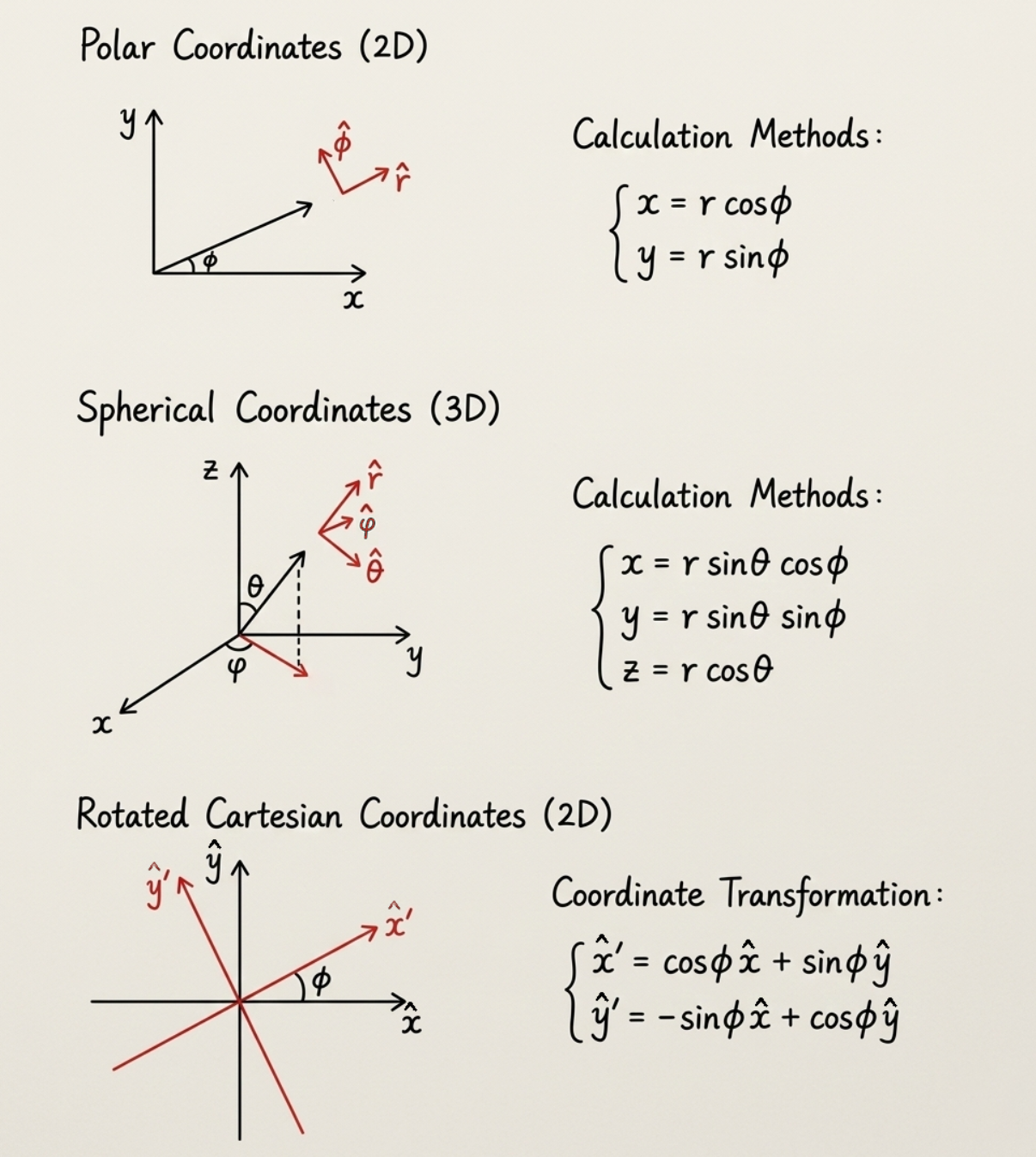
5. Vector Kinematic Definitions

• Position: \(\vec{r}\)

• Displacement: \(\Delta\vec{r} = \vec{r}_2 - \vec{r}_1\)

• Average Velocity:

  \[ \vec{v}_{avg} = \frac{\Delta\vec{r}}{\Delta t} = \frac{1}{\Delta t}\Delta\vec{r} \]

• Instantaneous Velocity:

  \[ \vec{v} = \lim_{\Delta t \to 0} \frac{\Delta\vec{r}}{\Delta t} = \frac{d\vec{r}}{dt} \]

• Average Acceleration:

  \[ \vec{a}_{avg} = \frac{\vec{v}_2 - \vec{v}_1}{t_2 - t_1} \]

• Instantaneous Acceleration:

  \[ \vec{a} = \lim_{\Delta t \to 0} \frac{\Delta\vec{v}}{\Delta t} = \frac{d\vec{v}}{dt} = \frac{d^2\vec{r}}{dt^2} \]

---

6. Kinematics by Component

This section breaks down the vector derivatives into their Cartesian components (\(\hat{i}, \hat{j}, \hat{k}\)).

• Position Vector:

  \[ \vec{r} = x\hat{i} + y\hat{j} + z\hat{k} \]

• Velocity Vector: Taking the derivative of the position vector with respect to time:

  \[ \Rightarrow \vec{v} = \frac{d\vec{r}}{dt} = \frac{dx}{dt}\hat{i} + \frac{dy}{dt}\hat{j} + \frac{dz}{dt}\hat{k} \]
  \[ = v_x\hat{i} + v_y\hat{j} + v_z\hat{k} \]

• Acceleration Vector: Taking the derivative of the velocity vector with respect to time:

  \[ \vec{a} = \frac{d\vec{v}}{dt} = a_x\hat{i} + a_y\hat{j} + a_z\hat{k} \]

---

7. Projectile Motion

This section applies the vector equations to standard 2D projectile motion.

• General Equations:

  \[ \vec{r} = \vec{r}_0 + \vec{v}_0t + \frac{1}{2}\vec{a}t^2 \]
  \[ \vec{a} = -g\hat{j} \]

• Solving for Range (\(s\)) and Time (\(t\)):

  Assuming the projectile starts at the origin and lands at a final position \(\vec{r}_f\) on the same horizontal level:

  \[ \vec{r}_f = s\hat{i} + 0\hat{j} \]

  Expressing this as column vectors:

  \[ \Rightarrow \binom{s}{0} = \binom{v_0\cos\phi_0 t}{v_0\sin\phi_0 t} + \frac{1}{2}\binom{0}{-gt^2} \]

• Results: Solving the \(y\)-component for \(t\) and substituting into the \(x\)-component yields:

  \[ t = \frac{2v_0\sin\phi_0}{g} \]
  \[ s = \frac{v_0^2\sin2\phi_0}{g} \]

---

8. Example: The Falling Target

This section analyzes a classic physics problem: aiming a projectile at a target that begins to fall from rest at the exact moment the projectile is fired.

• Problem Setup:

  • \(T\): Target position vector \(\vec{r}_{0T}\)

  • \(\phi_0\): Angle of the target relative to the origin.

  • \(\phi\): Aiming angle of the projectile.

  • \(Q_1\): Where to aim?

  • \(Q_2\): What is the minimal speed?

• Method 1: Reference Frame Change

  (Solving the problem by shifting to an accelerating frame of reference moving downward with gravity \(g\)).

• Method 2: Kinematic Equations Using the general equation \(\vec{r} = \vec{r}_0 + \vec{v}_0t + \frac{1}{2}\vec{a}t^2\):

  • Projectile Position (\(\vec{r}_{op}\)):

    \[ \vec{r}_{op} = \vec{v}_0t - \frac{1}{2}gt^2\hat{j} \]

  • Target Position (\(\vec{r}_{oT}\)):

    \[ \vec{r}_{oT} = (r_{0T}\cos\phi_0\hat{i} + r_{0T}\sin\phi_0\hat{j}) - \frac{1}{2}gt^2\hat{j} \]

  • Collision Condition (\(\vec{r}_{op} = \vec{r}_{oT}\)):

    Equating the two positions causes the gravity terms (\(-\frac{1}{2}gt^2\hat{j}\)) to cancel out:

    \[ \Rightarrow \vec{v}_0t = r_{0T}(\cos\phi_0\hat{i}) + r_{0T}\sin\phi_0\hat{j} \]

  • Conclusion:

    Expressing the velocity vector \(\vec{v}_0\) in terms of its angle \(\phi\):

    \[ t\binom{v_{0}\cos\phi}{v_{0}\sin\phi} = r_{0T}\binom{\cos\phi_0}{\sin\phi_0} \]
    \[ \Rightarrow \begin{cases} \phi = \phi_0 \\ t = r_{0T}/v_{0} \end{cases} \]

    (This proves that to hit the falling target, you must aim exactly at its initial position, \(\phi = \phi_0\).)

---

9. Uniform Circular Motion (Geometric Approach)

This section derives centripetal acceleration using the geometric properties of a circular path and limits.

• Definitions:

  • Acceleration definition: \(\vec{a} = \lim_{\Delta t \to 0} \frac{\Delta\vec{v}}{\Delta t}\)

  • Angle swept over time \(\Delta t\): \(\theta = \frac{v\Delta t}{r}\)

• Change in Velocity (\(|\Delta\vec{v}|\)): By looking at the vector triangle formed by initial and final velocities, the magnitude of the change in velocity is:

  \[ |\Delta\vec{v}| = 2v \sin\frac{\theta}{2} \]

• Magnitude of Acceleration (\(|\vec{a}|\)):

  Taking the limit as \(\Delta t \to 0\) (applying the small-angle approximation where \(\sin x \approx x\)):

  \[ |\vec{a}| = \lim_{\Delta t \to 0} \frac{2v \sin\frac{\theta}{2}}{\Delta t} = \lim_{\Delta t \to 0} \frac{2v \sin(\frac{v\Delta t}{2r})}{\Delta t} = \frac{v^2}{r} \]

• Vector Form: Because the acceleration points towards the center of the circle, it is expressed with the negative radial unit vector:

  \[ \vec{a} = -\frac{v^2}{r}\hat{r} \]

---

10. Formal Derivation Using Polar Coordinates

This section sets up the mathematical foundation for analyzing circular motion using polar basis vectors (\(\hat{r}\) and \(\hat{\phi}\)) instead of standard Cartesian ones (\(\hat{i}\) and \(\hat{j}\)).

• Basis Transformation Matrix:

  \[ \{\hat{r}, \hat{\phi}\} = \{\hat{i}, \hat{j}\} \begin{pmatrix} \cos\phi & -\sin\phi \\ \sin\phi & \cos\phi \end{pmatrix} \]

• Time Derivative of the Radial Vector (\(\hat{r}\)):

  Taking the derivative with respect to time \(t\) yields:

  \[ \frac{d\hat{r}}{dt} = \frac{d\cos\phi}{dt}\hat{i} + \frac{d\sin\phi}{dt}\hat{j} \]
  \[ = -\sin\phi \frac{d\phi}{dt}\hat{i} + \cos\phi \frac{d\phi}{dt}\hat{j} \]

  Substituting \(\hat{i}\) and \(\hat{j}\) back into their polar representations:

  \[ = -\sin\phi \frac{d\phi}{dt} (\cos\phi\hat{r} - \sin\phi\hat{\phi}) + \cos\phi \frac{d\phi}{dt} (\sin\phi\hat{r} + \cos\phi\hat{\phi}) \]

  Simplifying this gives the crucial result:

  \[ \frac{d\hat{r}}{dt} = \frac{d\phi}{dt}\hat{\phi} \]

• Time Derivative of the Angular Vector (\(\hat{\phi}\)):

  Similarly, taking the derivative of \(\hat{\phi}\) yields:

  \[ \frac{d\hat{\phi}}{dt} = -\frac{d\phi}{dt}\hat{r} \]

---

11. Uniform Circular Motion (Calculus Method)

Applying the polar coordinate derivatives to confirm the kinematics of uniform circular motion.

• Angular Velocity (\(\omega\)):

  \[ \frac{d\phi}{dt} = \omega = \frac{v}{r} \]

• Position Vector:

  \[ \vec{r} = r\hat{r} \]

• Velocity Vector: Taking the time derivative of position:

  \[ \Rightarrow \vec{v} = \frac{d\vec{r}}{dt} = r\frac{d\hat{r}}{dt} = r\frac{d\phi}{dt}\hat{\phi} = \omega r\hat{\phi} \]

• Acceleration Vector: Taking the time derivative of velocity:

  \[ \vec{a} = \frac{d\vec{v}}{dt} = \omega r\frac{d\hat{\phi}}{dt} = \omega r\left(-\frac{d\phi}{dt}\hat{r}\right) \]
  \[ = -\omega^2 r\hat{r} = -\frac{v^2}{r}\hat{r} \]

---

12. Non-Uniform Circular Motion

When the speed of the particle in the circular path is changing, the angular velocity \(\omega\) becomes time-dependent.

• Time-Dependent Angular Velocity:

  \[ \omega = \frac{d\phi}{dt} \quad \text{(Time dependent)} \]

• Velocity:

  \[ \vec{v} = \frac{d\vec{r}}{dt} = \omega r\hat{\phi} \]

• Acceleration (Applying the Product Rule):

  Because \(\omega\) is no longer constant, differentiating the velocity vector produces two terms:

  \[ \vec{a} = \frac{d\vec{v}}{dt} = \frac{d\omega}{dt}r\hat{\phi} + \omega r\frac{d\hat{\phi}}{dt} \]

  • \(\frac{d\omega}{dt}r\hat{\phi}\): This is the Tangential acceleration component (changes the speed).

  • \(\omega r\frac{d\hat{\phi}}{dt}\): This evaluates to \(-\omega^2r\hat{r}\), which is the Centripetal acceleration component (changes the direction).