Lecture 1: AVL Trees, Splay Trees, and Amortized Analysis
主线:Dynamic searching(动态查找)→ local restructuring(局部重构)→ complexity guarantees(复杂度保证)。 AVL 保证每次操作都快;Splay 允许个别操作慢,但控制整段操作的总成本。
Course overview(课程信息) · HW1 C implementation(编程题实现)
1. Dynamic searching(动态查找)
1.1 BST and tree shape(二叉搜索树与树形)
Binary search tree, BST(二叉搜索树): at every node, all left-subtree keys are smaller and all right-subtree keys are larger; both subtrees satisfy the same rule. Assume distinct keys, or specify a duplicate-key policy(重复键策略).
- Find / Insert / Delete: \(O(h+1)\), following a root-to-node path.
- Complete BST(完全二叉搜索树): \(h=\Theta(\log N)\).
- Sorted insertion(有序插入)into an ordinary BST: a chain with \(h=N-1\), hence \(O(N)\) operations.
- Dynamic data(动态数据)changes online: future keys are unknown. Sorting once + binary search(排序后二分查找)does not solve updates; ordered-array insertion/deletion may require \(O(N)\) shifts.
| Response | Idea | Guarantee / limitation |
|---|---|---|
| Arrange input order(调整输入顺序) | Insert medians first. | Good initial tree, but cannot control unknown future arrivals. |
| Treap(树堆,Tree + Heap) | BST order on keys + heap order on independent random priorities(随机优先级). | Expected(期望)height \(O(\log N)\) under sufficiently random priorities; extra storage/maintenance. |
| AVL: detect and repair(检测并修复) | Maintain a cheap invariant(不变量); fix violations locally. | Deterministic(确定性)\(O(\log N)\) worst-case operations. |
设计要点:“平衡”必须有可计算的指标和复杂度证明。Height balance(高度平衡)、black-height balance(黑高平衡)、weight balance(权重平衡)是不同约束。强制保持完全 BST 的固定形状可能造成大量重排;AVL 用少量不平衡换取便宜的更新。
1.2 ASL(平均查找长度)· MOOC Definition checkpoints
For equally likely successful searches(成功查找), one comparison per visited node:
Depth(深度)counts edges from the root. ASL here averages over stored keys in one fixed tree; it is not amortized analysis(摊还分析).
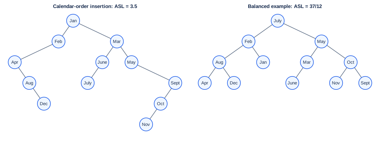
| Example / checkpoint | Calculation | Answer |
|---|---|---|
| Calendar-order insertion, Jan → Dec | Total comparisons / 12 | \(42/12=3.5\) |
| Q1: pictured balanced tree, root July | \((1+2\cdot2+4\cdot3+5\cdot4)/12\) | \(37/12\approx3.1\) |
| Q2: skewed(退化)12-node tree | \((1+2+\cdots+12)/12\) | \(6.5\) |
注意:month names are compared alphabetically(按字母顺序), not by calendar order. Balanced does not mean complete; balanced shapes can have different ASLs.
2. AVL trees(AVL 高度平衡树)
2.1 Definition and metadata(定义与辅助信息)
AVL = BST + recursive height balance(递归高度平衡), named after Adelson-Velskii and Landis (1962). Empty trees are balanced; a nonempty tree is balanced iff both subtrees are balanced and their heights differ by at most 1.
Balance factor, BF(平衡因子):左高减右高。 A leaf has height 0. Check every node: root BF = 0 does not imply AVL; visual asymmetry does not imply imbalance.
Store BF or cached height(缓存高度)per node; update locally in \(O(1)\) while recursion unwinds(递归回溯). Recomputing heights by traversing whole subtrees loses the logarithmic bound.
2.2 Insertion and rotations(插入与旋转)
Normal BST insertion → update bottom-up → repair the lowest unbalanced ancestor(最低失衡祖先).
- Troublemaker(肇因节点): inserted key that increases subtree height.
- Trouble finder(失衡发现者): first ancestor with BF = ±2 when moving upward.
- Classify the first two directions from the trouble finder toward the inserted key; the key may lie deeper.
| Case(失衡路径) | Repair(修复动作) |
|---|---|
| LL | Right rotation(右单旋)at the trouble finder. |
| RR | Left rotation(左单旋)at the trouble finder. |
| LR | Left rotation at its left child, then right rotation at the trouble finder. |
| RL | Right rotation at its right child, then left rotation at the trouble finder. |
易混点:RR 描述“右—右”的失衡路径,修复动作却是左旋;LL/RR 不是旋转方向。
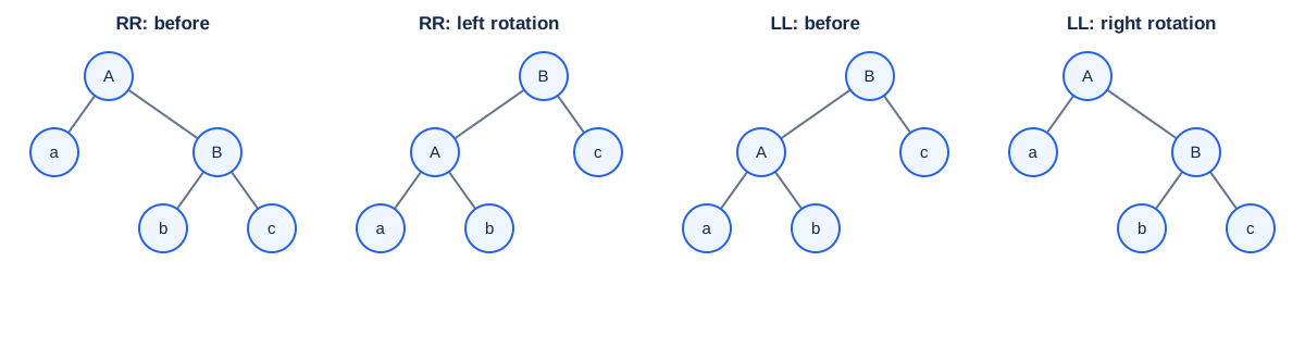
BST-order invariant(搜索顺序不变量): in RR, \(a<A<b<B<c\). Promote \(B\); its old left subtree \(b\) becomes \(A\)'s right subtree. Inorder order(中序顺序)is unchanged. LL is symmetric.
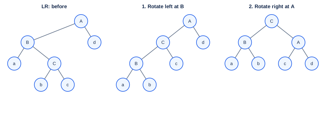
Double rotation(双旋): for LR, promote the middle key \(C\) between \(B\) and \(A\); preserve \(a<B<b<C<c<A<d\). \(C\)'s old left subtree goes to \(B\), its right subtree to \(A\). RL is symmetric; insertion in either subtree of \(C\) gives the same repair pattern.
Cost and locality(成本与局部性): each primitive rotation changes \(O(1)\) pointers/metadata. Reconnect the new subtree root to its parent, or replace the tree root. For insertion, repair restores the subtree's pre-insertion height(插入前高度), so ancestors need no further rotations: one repair site, at most two primitive rotations. Update metadata even when no rotation occurs.
Deletion(删除)区别: delete by the BST rule; for two children, replace by inorder predecessor/successor(中序前驱/后继). Update and rebalance upward. Height can decrease after repair, requiring \(O(\log N)\) repair sites; a heavy child's BF = 0 uses a single rotation. “一次局部修复即可”只适用于插入。
2.3 Month-name trace(月名插入)· rotation checkpoints
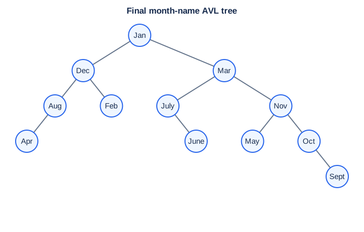
| Insert | Trouble finder | Case | Promoted root |
|---|---|---|---|
| Nov | Mar | RR | May |
| Apr | Mar | LL | Aug |
| Jan | May | LR | Mar |
| Feb | Aug | RL | Dec |
| June | Mar | LR | Jan |
| Oct | May | RR | Nov |
Other insertions, including Dec, July and Sept, need metadata updates but no rotations.
MOOC Single rotations Q1: where does \(B\)'s old left subtree go after RR? Right subtree of \(A\); its keys satisfy \(A<\text{keys}<B\).
Single rotations Q2: after inserting Apr, which nodes participate? Mar, Aug, Apr; Mar is the lowest trouble finder, repaired by LL. Repair it before considering higher ancestors.
Double rotations Q1: after inserting June, which statement is false?
- A. July is the parent of Jan.
- B. Jan is the root.
- C. Mar is the parent of May.
- D. Aug and Feb are siblings.
Answer: A. LR promotes Jan above Dec and Mar; Jan is an ancestor of July. At this stage Dec has children Aug/Feb and Mar still has right child May. 后续 Oct、Sept 会改变树形,不能用最终图判断中间阶段。
2.4 Height bound(高度界)· Quiz 1.1 Q2 / HW1 MC1
Let \(n_h\) be the minimum node count(最少节点数) of a height-\(h\) AVL tree. Minimal subtrees have heights \(h-1,h-2\):
where \(F_0=0,F_1=1\). The bases and recurrence follow by considering \(n_h+1\). With \(\varphi=(1+\sqrt5)/2\),
The leading base-2 coefficient is \(1/\log_2\varphi\approx1.44\). AVL may be taller than complete trees by a constant factor; Find/Insert/Delete are worst-case \(O(\log N)\).
Question: minimum nodes at tree depth 6, with empty depth −1? A. 13; B. 17; C. 20; D. 33.
| \(h\) | −1 | 0 | 1 | 2 | 3 | 4 | 5 | 6 |
|---|---|---|---|---|---|---|---|---|
| \(n_h\) | 0 | 1 | 2 | 4 | 7 | 12 | 20 | 33 |
Answer: D, \(n_6=1+20+12=33\). Here tree depth means height(最大节点深度).
下标警告:empty height −1 / leaf height 0 → \(F_{h+3}-1\); empty height 0 / leaf height 1 → \(F_{h+2}-1\). 视频和课件的下标不完全一致,先核对高度约定。
3. Splay trees(伸展树)
3.1 Target(目标)
Self-adjusting BST(自调整二叉搜索树): splay the accessed node to the root; no BF/height field is needed for balance maintenance. The tree need not remain height-balanced.
For \(M\) operations starting empty, with at most \(N\) keys present:
The lecture writes \(O(M\log N)\); \(+1\) handles empty/singleton sets. A single operation can cost \(\Theta(N)\), but the next access to the same root key is \(O(1)\).
MOOC Target T/F: “An AVL tree is a splay tree.” Course answer: True, meaning AVL satisfies the same sequence-cost target. As a data-structure definition: False; AVL and splay are different algorithms. 复杂度保证蕴含 ≠ 数据结构等同。
3.2 Move-to-root fails(朴素移至根策略的反例)
Repeatedly rotating the accessed node with its parent is insufficient. Insert \(1,\ldots,N\) with this rule: \(O(N)\) total, yielding a left chain rooted at \(N\). Then access \(1,\ldots,N\): the chain returns after each sweep, with \(\Theta(N^2)\) total work.
Comparison count: Find(1) costs \(N\); Find(\(i\ge2\)) costs \(N-i+2\):
MOOC Single rotations checkpoint: complexity of these \(N\) finds? \(\Theta(N^2)\), option C. Exported option images are blank; the video/slides explicitly state the quadratic result. 只让当前节点变浅,可能把其他节点压深;必须控制旋转顺序。
3.3 Splaying steps(伸展步骤)
Let \(x\) be accessed, \(p\) its parent(父节点), \(g\) its grandparent(祖父节点). Repeat bottom-up(自底向上) until \(x\) is root:
| Case | Condition | Rotation order |
|---|---|---|
| Zig(单旋) | \(p\) is root | Rotate \(x\) with \(p\); terminal step(最后一步). |
| Zig-zag(异向双旋) | \(x,p\) on opposite sides | Rotate \(x\) with \(p\), then \(x\) with \(g\). |
| Zig-zig(同向双旋) | \(x,p\) on the same side | Rotate \(p\) with \(g\) first, then \(x\) with \(p\). |
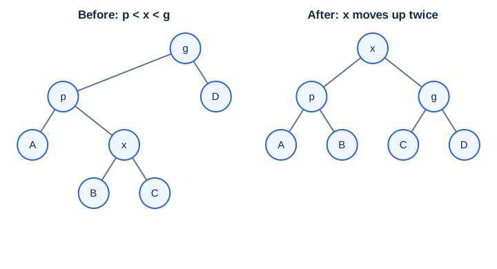
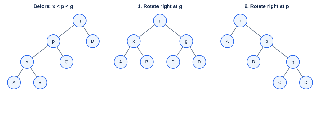
易错:Zig-zig 先转父节点与祖父节点,不能先转 \(x,p\)。Zig-zig 和 zig-zag 都包含 two primitive rotations(两次基本旋转);课件的 “single rotation” 标签不代表 zig-zig 只转一次。
Reconnect hanging subtrees(挂接子树), the tree root, and parent pointers if used. Parent pointers or an explicit path stack(路径栈)can support bottom-up updates.
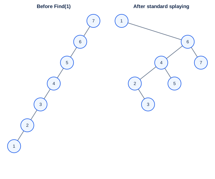
Splaying roughly shortens depths along the access path(访问路径); the 7-node and textbook 32-node examples illustrate this. 不是每个节点深度或全树高度都必然减半;保证来自摊还证明。
3.4 Operations(操作)
| Operation | Procedure |
|---|---|
| Find | BST search, then splay the found node; on failure, splay the last visited node if nonempty. |
| FindMin / FindMax | Find and splay the extreme key(最小/最大键). |
| Insert | BST leaf insertion, then splay the new node; under set semantics, splay an existing duplicate without adding a copy. |
| Delete | Find/splay target → remove root → join remaining subtrees(合并子树). |
Deletion/join: if either subtree is empty, return the other. Otherwise splay \(\max(L)\) in the left subtree; it has no right child. Attach the old right subtree \(R\) there. All \(L\) keys are smaller than all \(R\) keys, preserving BST order. Symmetrically, splay \(\min(R)\) and attach \(L\) on the left. Clear/set parent links when detaching/attaching.
Quiz 1.2 Q2: “Finding the maximum leaves the root with no right subtree.” True when FindMax includes splaying: any right child would contradict maximality(最大性).
3.5 AVL vs. Splay(比较)
| Property | AVL | Splay |
|---|---|---|
| Shape invariant(树形约束) | Recursive height balance | BST order only |
| Balance metadata(平衡辅助信息) | BF / height | None; still needs parent/path machinery |
| Successful find | No restructuring | Splays unless already root |
| Worst case per operation(单次最坏情况) | \(O(\log N)\) | \(O(N)\) |
| Amortized standard operations(摊还界) | \(O(\log N)\) | \(O(\log N)\) |
| Tradeoff(取舍) | Predictable latency(延迟) | Access locality(访问局部性), but more writes/rotations |
Benchmark random/sorted inputs, hot keys(热点键), failed searches, and mixed updates; measure comparisons, rotations, total time, and maximum latency. Splay is not universally faster; amortized guarantees do not ensure real-time(实时)per-request bounds. 线下“AVL 已不使用”的说法不宜当作普遍事实。
4. Amortized analysis(摊还分析)
4.1 What is bounded?(保证的对象)
| Bound | Meaning | Probability assumptions(概率假设) |
|---|---|---|
| Worst-case(最坏情况) | Every individual operation | None |
| Amortized(摊还) | Total cost of every valid sequence, divided by its length | None |
| Average-case(平均情况) | Expected cost under a specified distribution(分布) | Required |
For the same cost model, worst-case per-operation guarantee → amortized sequence guarantee → expected sequence bound under any distribution. 课件的 “≥” 表示保证强弱,不是不同复杂度函数之间的数值比较。
Example: deterministic quicksort averages \(O(N\log N)\) over equally likely permutations(等概率排列), but can take \(O(N^2)\). Amortized analysis controls expensive operations through their history, without random-input assumptions.
Quiz 1.3 Q2: amortized \(O(\log N)\) implies worst-case \(O(\log N)\)? False; a splay access can be linear.
4.2 Stack + MultiPop(栈与批量弹出): three methods
For \(k\ge0\), let \(k'=\min(k,|S|)\). Count each elementary push/pop as 1: MultiPop removes \(k'\) objects. With call/loop overhead, runtime is \(\Theta(1+k')\).
Aggregate analysis(聚合分析): in \(m\) operations on an empty stack, each pushed object is popped at most once. With \(P\le m\) pushes, total element work \(\le2P\le2m\), hence amortized \(O(1)\). For \(m\ge2\), \(m-1\) pushes + one MultiPop gives \(2m-2\) units. Repeating MultiPop on empty cannot repeat expensive removal. With \(s_0\) initial objects, the bound becomes \(O(m+s_0)\).
Accounting method(记账法): charge \(\widehat c_i\), pay actual cost \(c_i\), and store the difference as credit(预存额度). Credit must stay nonnegative after every prefix(每个操作前缀):
| Operation | \(c_i\) | \(\widehat c_i\) | Credit change |
|---|---|---|---|
| Push | 1 | 2 | +1 |
| Successful Pop | 1 | 0 | −1 |
| MultiPop | \(k'\) | 0 | \(-k'\) |
One credit per stored object → credit = stack size ≥ 0 → total charge \(2P=O(m)\). 零摊还成本不是零实际时间,而是此前已付费。 Add constant charges for call overhead. The offline alternative charges 3/1/1 also work, but give a looser \(O(m)\) bound; charges are not unique. Aggregate gives a uniform average; accounting can assign different charges to different operations.
Potential method(势能法): state \(D_i\) after operation \(i\); potential function(势函数)\(\Phi\) stores credit in the whole state:
Telescoping(望远镜求和)cancels intermediate potentials. If \(\Phi(D_j)\ge\Phi(D_0)\) for every prefix, charges upper-bound actual cost. Common normalization(归一化): \(\Phi(D_0)=0\), \(\Phi\ge0\). Potential may rise/fall; an additive constant does not change charges. 初始势能不为最小值时,必须保留边界项。
For the stack, \(\Phi(D)=|S|\): changes \(+1,-1,-k'\) reproduce charges \(2,0,0\).
HW1 MC4: which statement is false?
- A. Aggregate analysis yields \(T(m)/m\) from a worst-case sequence total \(T(m)\).
- B. A good potential should always attain its maximum initially.
- C. Accounting saves excess charges for later expensive operations.
- D. Accounting allows operation charges to differ, unlike the uniform aggregate average.
Answer: B. An initial minimum(最小值) provides the usual upper-bound condition; the actual requirement is the boundary-term inequality.
5. Splay amortized proof(伸展树的摊还证明)
5.1 Rank and potential(秩与势能)
For a fixed node set, subtree size includes the node itself:
Rank(秩)≠ height(高度); leaf rank = 0. Rank/potential are analysis tools and need not be stored. A rotation changes ranks only at the two/three main nodes; hanging subtrees and ancestor subtree sizes stay unchanged.
Log lemma(对数引理): for positive \(a,b,c\), \(a+b\le c\) implies \(ab\le c^2/4\) by AM–GM(算术—几何平均不等式):
The −2 uses base-2 logs. Subtree sizes are additive; heights are not. Replacing rank by height breaks this argument.
5.2 Local costs(局部成本)
Use \(r\) before, \(r'\) after; one primitive rotation costs 1. Let \(\Delta=r'(x)-r(x)\ge0\).
Zig: \(r'(p)\le r(p)\), so
For either two-rotation case, \(r'(x)=r(g)\) and \(r(p)\ge r(x)\):
| Case | Key size/rank relation | Amortized bound |
|---|---|---|
| Zig-zag | \(s'(p)+s'(g)\le s'(x)\) → \(r'(p)+r'(g)\le2r'(x)-2\) | \(\widehat c\le2+2r'(x)-2-2r(x)=2\Delta\) |
| Zig-zig | Old \(x\) subtree and new \(g\) subtree are disjoint: \(s(x)+s'(g)\le s'(x)\) → \(r(x)+r'(g)\le2r'(x)-2\); also \(r'(p)\le r'(x)\) | \(\widehat c\le2+r'(x)+r'(g)-2r(x)\le3\Delta\) |
Mirror cases(镜像情形)are identical. 关键不是让每次实际成本都小,而是让秩的变化支付昂贵旋转。
5.3 Access lemma(访问引理)and boundary terms(边界项)
All nonterminal steps cost at most \(3\Delta\); only a final zig contributes +1. Consecutive rank differences of \(x\) telescope. With original root \(t\),
This bounds rotation cost + potential change, not actual cost of one access. Search depth and rotation work are proportional, up to constants. Standard steps and the access lemma are corroborated by Sleator–Tarjan, Section 2.
Initial state matters(初始状态很重要): \(0\le\Phi(T)\le N\log_2N\), but an arbitrary initial tree need not minimize potential. For \(M\) accesses,
Starting empty removes initial credit. For updates, insertion can be implemented as splay-last-search-node → split → new root: the new root adds at most \(\log(N+1)\) rank, retained roots do not gain size. Deletion splays/removes the target, splays \(\max(L)\), then attaches \(R\); attaching changes one root rank by at most \(\log(N+1)\). Together with the access lemma this gives logarithmic amortized updates; leaf-insert-then-splay also has the standard guarantee.
课件澄清:“势能在 \(N\) 步内最多增加 \(O(\log N)\)”不是总势能必须满足的条件。\(\Phi\) 可以为 \(\Theta(N\log N)\);要控制的是每次操作的 \(c_i+\Delta\Phi_i\),以及初末边界项。
6. Integrated exercises(综合题)
6.1 AVL insertion(AVL 插入)· Quiz 1.1 Q1 / HW1 MC2
Insert \(2,1,4,5,9,3,6,7\) into an empty AVL tree. Which is false?
- A. 4 is the root.
- B. 3 and 7 are siblings(兄弟节点).
- C. 2 and 6 are siblings.
- D. 9 is the parent of 7.
Only three repairs: insert 9 → RR at 4; insert 3 → RL at 2; insert 6 → RL at 5. Root sequence: \(2,2,2,2,2,4,4,4\).
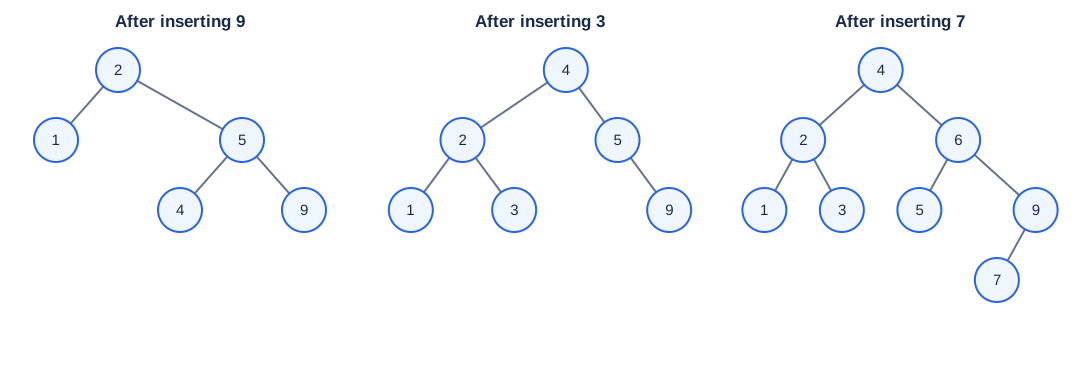
Answer: B. Final children: 4 → (2,6), 2 → (1,3), 6 → (5,9), 9 → (7,∅). 3 的父节点是 2,7 的父节点是 9。
6.2 Splay accesses(伸展树访问)· Quiz 1.2 Q1 / HW1 MC3
Access \(3,9,1,5\) in order in the following tree. Which final statement is false?
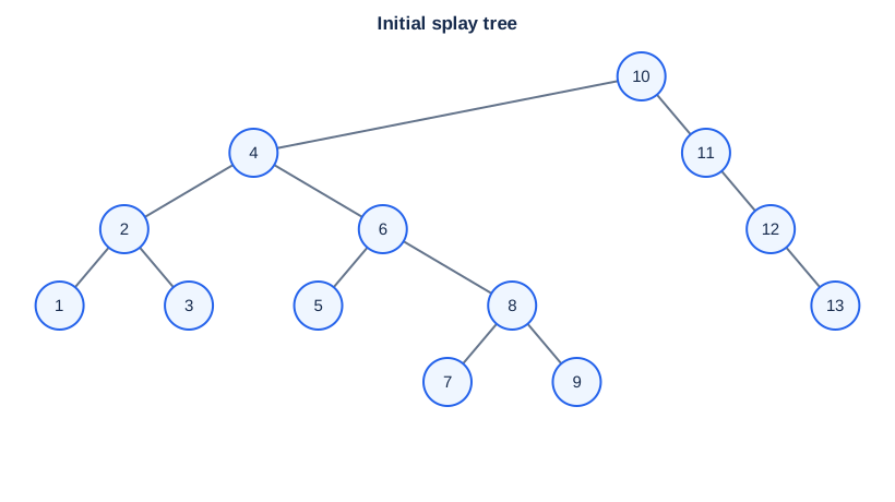
- A. 5 is the root.
- B. 1 and 9 are siblings.
- C. 6 and 10 are siblings.
- D. 3 is the parent of 4.
| Access | Steps, from bottom upward |
|---|---|
| 3 | Zig-zag (3,2,4); zig (3,10). |
| 9 | Zig-zig (9,8,6); zig-zag (9,4,10); zig (9,3). |
| 1 | Zig-zig (1,2,3); zig (1,9). |
| 5 | Zig-zig (5,6,8); zig-zig (5,4,3); zig-zag (5,2,9); zig (5,1). |
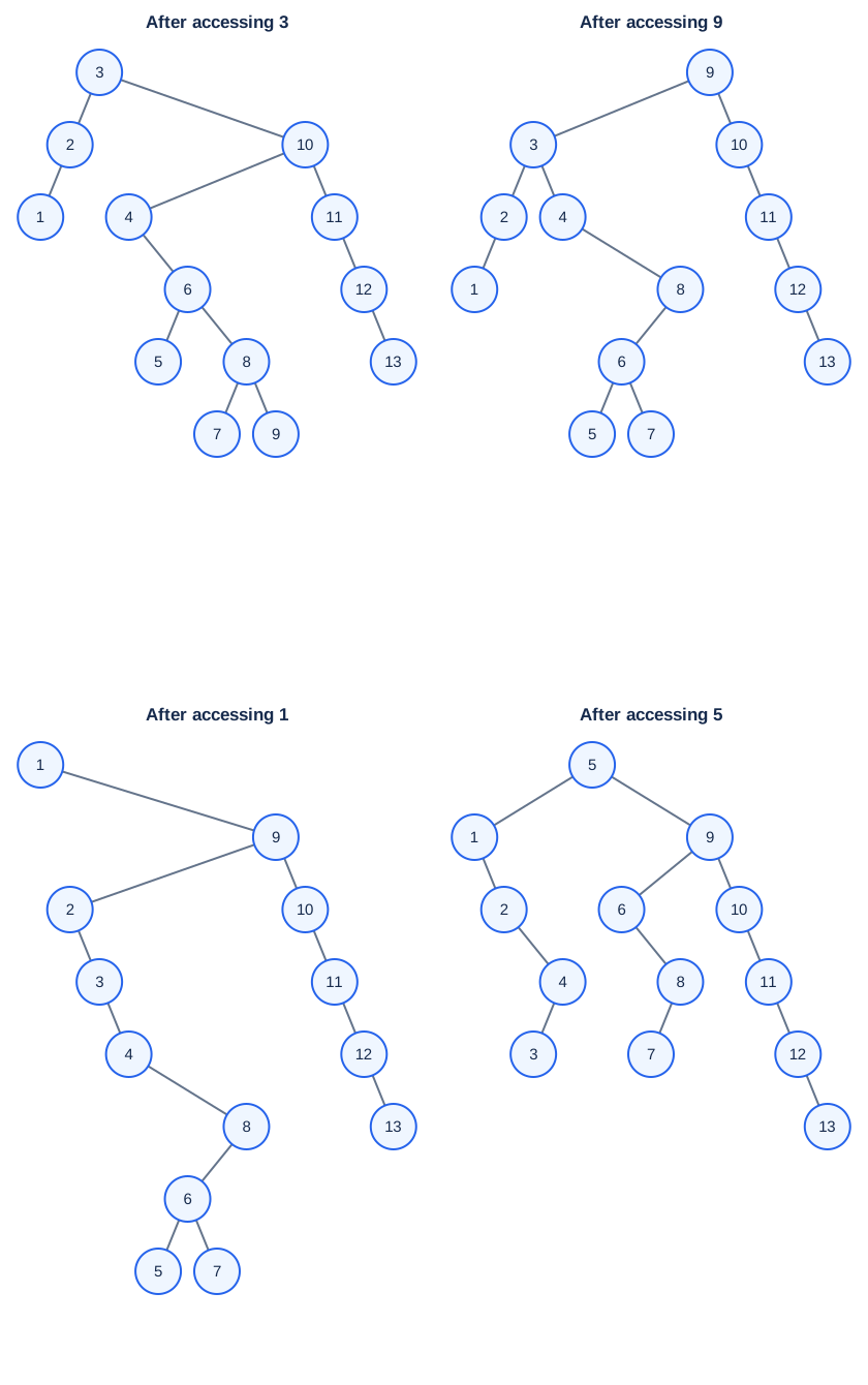
Answer: D. Final relationships: 5 → (1,9), 9 → (6,10), 4 has left child 3. Each accessed key becomes root; the remaining 10 → 11 → 12 → 13 chain shows that splay need not produce AVL balance.
6.3 Buffer doubling(缓冲区倍增)· Quiz 1.3 Q1 / HW1 MC5
Problem: initially empty, capacity 1. Insertion costs 1 if space exists; otherwise copy \(k\) old items into a doubled buffer and insert, costing \(k+1\). A single insertion can cost \(\Omega(N)\). Assume the buffer is full after \(N\) insertions. Which potential works?
- A. Number of items.
- B. Negative number of items.
- C. Number of available blocks.
- D. Negative number of available blocks.
Answer: D. With occupancy(已用数量)\(n\) and capacity(容量)\(C\), use \(\Phi=n-C\):
| Case | State change | \(c_i\) | \(\Delta\Phi\) | \(\widehat c_i\) |
|---|---|---|---|---|
| Space available | \((n,C)\to(n+1,C)\) | 1 | 1 | 2 |
| Resize(扩容) | \((k,k)\to(k+1,2k)\) | \(k+1\) | \(1-k\) | 2 |
Initially \(\Phi=-1\); at the full endpoint \(\Phi=0\), giving
Check by aggregate analysis: for power-of-two \(N\), copied items \(1+2+\cdots+N/2=N-1\), plus \(N\) writes. A/B/C give resizing charges \(k+2,k,2k\), respectively, so none cancels copying to a constant.
易错:D 的势能在中途可以低于初值,所以 \(2j\) 不保证覆盖任意前缀;题目的“最终装满”条件不能省略。For all prefixes, choose \(\Psi=2n-C+1\): initially 0, nonnegative thereafter, and every insertion has charge 3. Thus arbitrary \(N\) insertions cost at most \(3N\); geometrically summing copies also gives total cost \(<3N\).
6.4 HW1 programming(编程题): Root of AVL Tree
Task: read \(1\le N\le20\) distinct integer keys, insert in order, print the final root. Cache heights; recursively insert and rebalance; update the demoted node before the promoted node.
88 70 61 96 120→ root 70: LL at 88 after 61; RR at 88 after 120.88 70 61 96 120 90 65→ root 88: RL at 70 after 90; 65 leaves the root unchanged.- Total time \(O(N\log(N+1))\); node storage \(O(N)\); recursion depth \(O(\log(N+1))\).
- Test all rotation cases, repairs below root, singleton, sorted/reversed keys, and \(N=20\).
Complete problem, sample I/O and tested C solution(完整题目、样例与 C 实现)
6.5 Week 2 review questions(第二周复习题)
以下题目来自第二周小测,只涉及本课知识;第二课时的新知识题按知识点另行整理。
WK2 MC1: delete 3 from the following splay tree; which statement is impossible? Input: 7(5(2(1,3(∅,4)),6),9(8,∅)).
- A. 2 is root.
- B. 4 is root.
- C. 6 and 9 are siblings.
- D. 4 is the grandparent of 5.
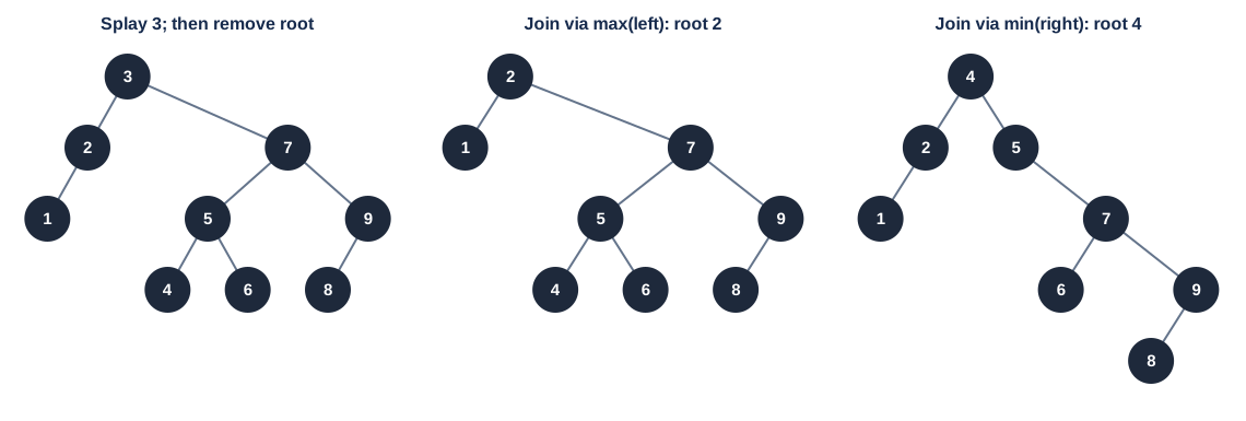
Answer: D. Splay 3 by zig-zag (3,2,5), then zig (3,7); remove root 3. Two joins(拼接)are valid:
| Join choice | Result | Options |
|---|---|---|
| Splay max(left) = 2; attach right subtree | 2(1,7(5(4,6),9(8,∅))) |
A possible; 4 is a child of 5. |
| Splay min(right) = 4; attach left subtree | 4(2(1,∅),5(∅,7(6,9(8,∅)))) |
B and C possible; 4 is the parent, not grandparent, of 5. |
易错:先伸展再删除,然后在剩余的一侧伸展极值;不能直接用普通 BST 的替换删除。题目没有指定哪种 join,“impossible”须检查两种合法结果。
WK2 MC2: in an AVL tree of height 4, what is the maximum difference between left/right subtree sizes? Choices A 1 / B 2 / C 3 / D 5.
Answer: D, 5, using this question's height = number of levels(高度按层数): leaf height 1, empty height 0. One root subtree can have height 3 and be full with \(2^3-1=7\) nodes; the other can have height 2 with its minimum 2 nodes. Difference \(7-2=5\). If both subtrees have height 3, maximum difference is \(7-4=3\), so 5 is the overall maximum.
注意题目换了高度约定:按本笔记 AVL 的边数高度,这棵树高度为 3。若真的按边数高度 4 计算,答案是 \(15-4=11\),不在选项中。AVL 约束的是高度差,不是节点数差。
WK2 MC3: which amortized-analysis statement is false?
- A. A good potential should always assume its maximum at the start.
- B. Accounting saves excess amortized charges as credit for later operations.
- C. Aggregate analysis bounds total \(T(n)\) for every sequence length \(n\), giving \(T(n)/n\) per operation.
- D. Accounting can assign different amortized costs to different operations, unlike the uniform aggregate average.
Answer: A. Same concept as HW1 MC4 in §4.2, with reordered options. Usually normalize the initial potential to a minimum and require \(\Phi(D_j)\ge\Phi(D_0)\) to upper-bound actual prefix costs. 不要沿用上一份题目的选项字母。
WK2 programming fill-in: RR rotation(右右失衡修复). Fill the pointer reassignment and new-root height in the given AVL function. The archive mixes Tree L, variable R, and return L: 变量名笔误; use R consistently.
Tree RR_Rotation(Tree T)
{
    Tree R = T->right;
    T->right = R->left;
    R->left = T;  /* blank 1 */
    T->h = maxh(Height(T->left), Height(T->right)) + 1;
    R->h = maxh(Height(R->left), Height(R->right)) + 1; /* blank 2 */
    return R;
}
The blanks are R->left = T and maxh(Height(R->left), Height(R->right)); the latter can use T->h for Height(R->left) after updating T. RR needs a left rotation(左旋); update the demoted node before the promoted node. Time and extra space: \(O(1)\); requires T != NULL and T->right != NULL.
7. Review and references(复习与来源)
复习重点:最低失衡祖先;旋转后中序顺序与子树高度;Fibonacci 下标;zig-zig 顺序;删除时的 join;单次最坏界与摊还界;credit / potential 的非负条件;rank 引理和望远镜求和;缓冲区题的最终装满条件。
These notes retain all 13 MOOC checkpoint/quiz questions and all six HW1 questions; duplicated questions share one solution. They also include the offline Treap, local-repair, implementation, and proof discussions. Sources: supplied lesson exports and merged indices (units 1320673500–1320673518), lecture-record-15/course_content.md and its 169 slide captures, and archived ZJUADS_cy2026_HW1.md. Course/project requirements are summarized on the course page.
- ZJU MOOC, supplied term 1488053496.
- Weiss, Data Structures and Algorithm Analysis in C, 2nd ed.: Chapter 4 pp. 106–128; Chapter 11 pp. 447–451. Figures 4.42–4.48 for code, 4.52–4.60 for larger splay examples.
- Cormen et al., Introduction to Algorithms, 3rd ed.: pp. 451–478. Page ranges follow the supplied slides.
- Sleator and Tarjan, Self-Adjusting Binary Search Trees (1985), Section 2.
The ten original Lecture 1 figures and the added WK2 deletion figure are editable SVG redrawings; question trees follow the supplied diagrams, with resulting states recomputed. Status remains draft pending textbook/instructor review.