07_Sinusoidal Waves

1. Sinusoidal Waves

The displacement \(y\) of a sinusoidal wave is given by the equation:

\[ y = A \sin(kx - \omega t + \phi) \]

Where:

• \(A\) = Amplitude

• \(k\) = Angular wave number

• \(\omega\) = Angular frequency

• \(\phi\) = Phase constant

Wave Parameters and Relations:

• Wave Number: \(k = \frac{2\pi}{\lambda}\)

• Angular Frequency: \(\omega = \frac{2\pi}{T}\)

• Wave Speed (Phase Velocity): From the argument \(x - vt \implies v = \frac{\omega}{k} = \frac{\lambda}{T}\)

Substituting these relations, the wave equation can also be written as:

\[ y = A \sin\left[ \frac{2\pi}{\lambda}(x - vt) + \phi \right] \]

Transverse Velocity and Acceleration:

• Velocity: \(v_y = \frac{\partial y}{\partial t} = -\omega A \cos(kx - \omega t + \phi)\)

• Acceleration: \(a_y = \frac{\partial^2 y}{\partial t^2} = -\omega^2 A \sin(kx - \omega t + \phi)\)

---

2. Rate of Energy Transfer

Kinetic Energy (\(K\)):

For a small mass element \(dm = \mu dx\) (where \(\mu\) is linear mass density):

\[ dK = \frac{1}{2} dm v_y^2 = \frac{1}{2} (\mu dx) \omega^2 A^2 \cos^2(kx - \omega t + \phi) \]

The rate of kinetic energy transfer is:

\[ \frac{dK}{dt} = \frac{1}{2} \mu v \omega^2 A^2 \cos^2(kx - \omega t + \phi) \]

Note: While displacement \(y \sim \sin(\dots)\), the kinetic energy rate \(\frac{dK}{dt} \sim \cos^2(\dots)\). The kinetic energy travels along with the wave.

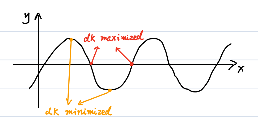
• schematic diagram from the hand-written notes of Mr. ztWang

Average Kinetic Energy Rate:

Since the average value of \(\cos^2\) over one period is \(\frac{1}{2}\) (i.e., \(\int_0^T \cos^2(\omega t) dt / \int_0^T dt = \frac{1}{2}\)):

\[ \left( \frac{dK}{dt} \right)_{avg} = \frac{1}{4} \mu v \omega^2 A^2 \]

• \(\frac{dK}{dt}\) is maximized when \(y = 0\) (element moving fastest).

• \(\frac{dK}{dt}\) is minimized when \(y = \pm A\) (element momentarily at rest).

Potential Energy (\(U\)):

The string is most stretched at \(y = 0\) (yielding maximum potential energy) and least stretched at the peaks \(y = \pm A\) (yielding minimum potential energy).

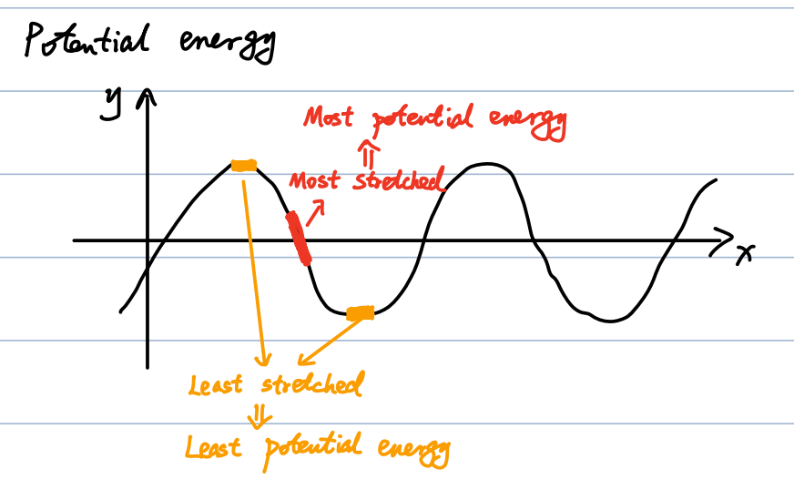
• Key Insight: The energy distribution for kinetic and potential energy is exactly the SAME!

  \[ \left( \frac{dU}{dt} \right)_{avg} = \frac{1}{4} \mu v \omega^2 A^2 \]

Total Average Power:

\[ P_{avg} = \left( \frac{d(K+U)}{dt} \right)_{avg} = \frac{1}{2} \mu v \omega^2 A^2 \]

---

3. Wave Interference

Given two waves:

\[ y_1 = A \sin(kx - \omega t) \]

\[ y_2 = A \sin(kx - \omega t + \phi) \]

By the principle of superposition (\(y = y_1 + y_2\)):

\[ y = 2A \cos\left(\frac{\phi}{2}\right) \sin\left(kx - \omega t + \frac{\phi}{2}\right) \]

Conditions for Interference:

1. Constructive Interference (in phase): \(\cos(\frac{\phi}{2}) = \pm 1 \implies \phi = 2\pi n\).

   Resulting wave: \(y = \pm 2A \sin(kx - \omega t + \frac{\phi}{2})\)

2. Destructive Interference (out of phase): \(\cos(\frac{\phi}{2}) = 0 \implies \phi = 2\pi(n + \frac{1}{2})\).

   Resulting wave: \(y = 0\)

Spatial Path Difference (\(\Delta r\)):

If two waves travel different distances (\(r_1\) and \(r_2\)) from a source, the path difference determines the phase difference (\(k\Delta r = \phi\)).

• Constructive: \(\Delta r = |r_1 - r_2| = n\lambda\)

• Destructive: \(\Delta r = |r_1 - r_2| = (n + \frac{1}{2})\lambda\)

---

4. Temporal Interference and Beats

Consider two waves with different frequencies and wave numbers, but assuming equal wave speed \(v_1 = v_2 = v\) (i.e., \(\frac{\omega_1}{k_1} = \frac{\omega_2}{k_2} = v\)):

\[ y_1 = A \sin(k_1 x - \omega_1 t + \phi_1) \]

\[ y_2 = A \sin(k_2 x - \omega_2 t + \phi_2) \]

Superposition yields:

\[ y = \left\{ 2A \cos\left[ \frac{\Delta\omega}{2}\left(\frac{x}{v} - t\right) + \frac{\phi_1 - \phi_2}{2} \right] \right\} \sin\left[ \omega_{avg}\left(\frac{x}{v} - t\right) + \frac{\phi_1 + \phi_2}{2} \right] \]

Where \(\omega_{avg} = \frac{\omega_1 + \omega_2}{2}\) and \(\Delta\omega = \omega_1 - \omega_2\).

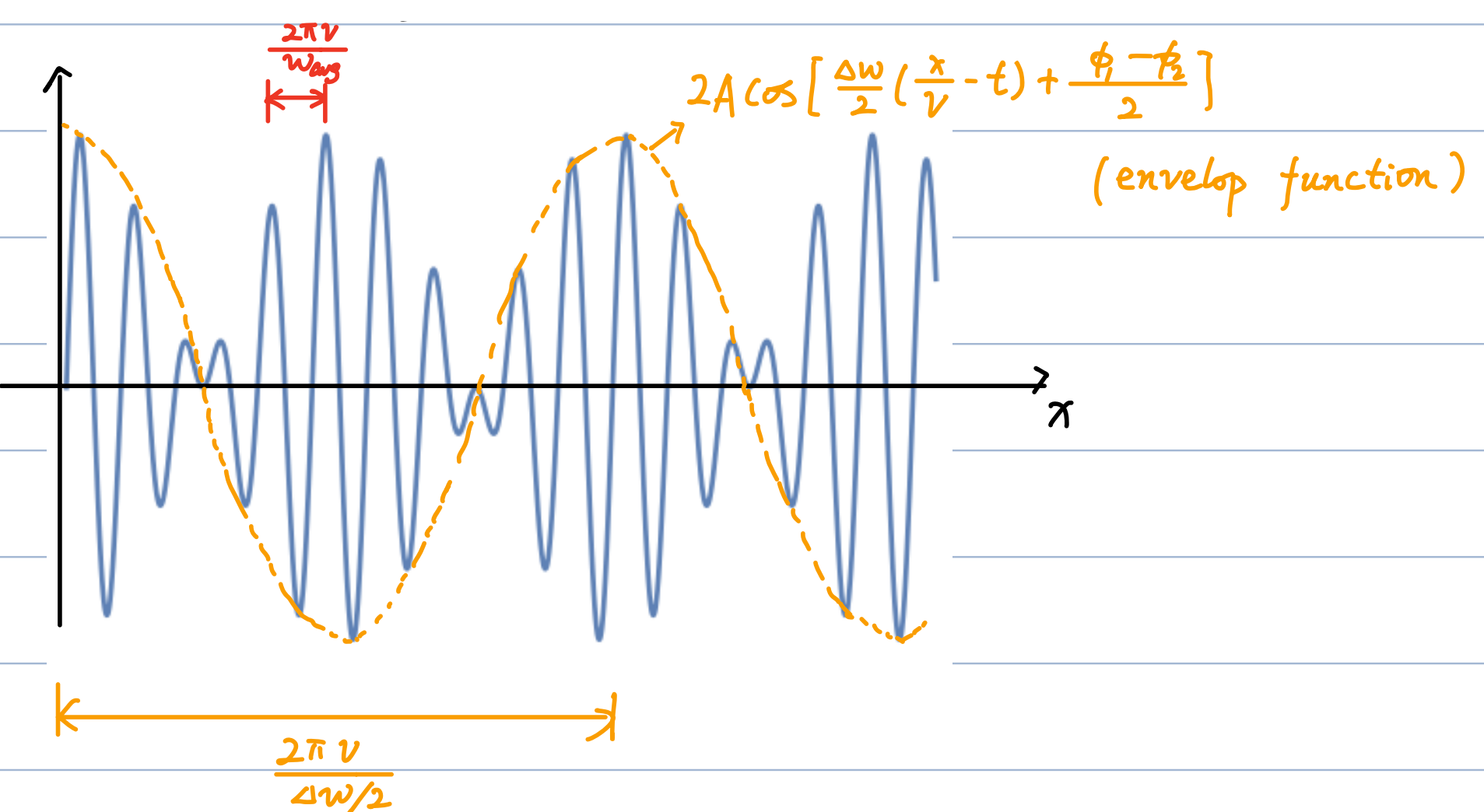
Assuming \(\omega_{avg} \gg |\Delta\omega|\) (frequencies are close, \(\omega_1 \approx \omega_2\)):

• The high-frequency carrier wave has a short wavelength: \(\lambda \sim \frac{2\pi v}{\omega_{avg}}\).

• The modulating envelope function has a long wavelength: \(\lambda' \sim \frac{2\pi v}{\Delta\omega / 2}\).

• Beat Frequency: \(f_{beat} = \frac{1}{2\pi} |\omega_1 - \omega_2| = |f_1 - f_2|\).

---

5. Group Velocity and Dispersion

If we no longer assume \(v_1 = v_2\), the superposition becomes:

\[ y = 2A \cos\left( \frac{\Delta k}{2} x - \frac{\Delta \omega}{2} t + \frac{\Delta \phi}{2} \right) \sin(k_{avg} x - \omega_{avg} t + \phi_{avg}) \]

• Phase Velocity: \(v_p = \frac{\omega}{k}\) (velocity of the individual wave peaks).

• Group Velocity: \(v_g = \frac{\Delta \omega}{\Delta k}\) (velocity of the envelope function). In the differential limit as \(\Delta\omega, \Delta k \to 0\), \(v_g = \frac{d\omega}{dk}\).

Dispersion Relations:

Based on the \(\omega\) vs. \(k\) curve:

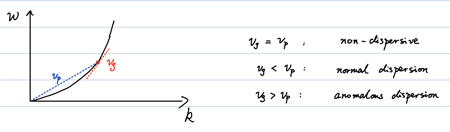
• \(v_g = v_p\): Non-dispersive

• \(v_g < v_p\): Normal dispersion

• \(v_g > v_p\): Anomalous dispersion

---

6. Standing Waves

When two identical waves travel in opposite directions:

\(y_1 = A \sin(kx - \omega t)\)

\(y_2 = A \sin(kx + \omega t)\)

Superposition yields:

\[ y = y_1 + y_2 = 2A \sin(kx) \cos(\omega t) \]

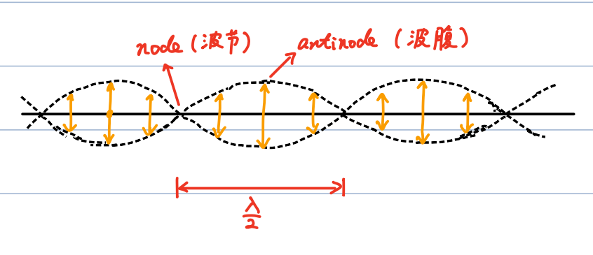
Characteristics:

• Nodes (波节): Points of zero amplitude. Occur when \(kx = n\pi \implies x = \frac{n}{2}\lambda\).

• Antinodes (波腹): Points of maximum amplitude. Occur when \(kx = (n + \frac{1}{2})\pi \implies x = (\frac{n}{2} + \frac{1}{4})\lambda\).

• Distance between adjacent nodes is \(\frac{\lambda}{2}\).

• There is just local oscillation; no wave propagation occurs.

• No energy is transmitted across a node.

Harmonic Series for String Fixed at Both Ends:

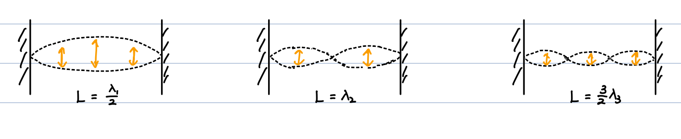
For a string of length \(L\):

• Wavelengths: \(\lambda_n = \frac{2L}{n}\) (for \(n = 1, 2, 3, \dots\))

• Frequencies: \(f_n = \frac{v}{\lambda_n} = n \frac{v}{2L}\)

Musical Sound Qualities:

• Pitch: Determined by fundamental frequency.

• Loudness: Determined by amplitude.

• Timbre (Tone Quality): Determined by the spectrum of harmonic overtones.

---

7. Fourier Analysis

Any periodic function \(f(t)\) with period \(T = \frac{2\pi}{\omega}\) (meaning \(f(t) = f(t+T)\)) can be expanded into a Fourier series. For example, a square wave of period \(T\) is constructed from harmonics with periods \(T, \frac{T}{3}, \frac{T}{5}, \dots\)

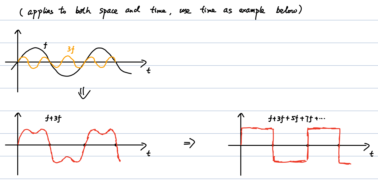
Fourier Series Expansion:

\[ f(t) = B_0 + \sum_{n=1}^{\infty} A_n \sin(n\omega t) + \sum_{n=1}^{\infty} B_n \cos(n\omega t) \]

Calculating Coefficients (\(A_n, B_n, B_0\)):

Using orthogonality properties where \(\frac{2}{T} \int_0^T \sin(m\omega t) \sin(n\omega t) dt = \delta_{m,n}\) (for \(m, n \ge 1\)):

• \(B_0 = \frac{1}{T} \int_0^T f(t) dt\)

• \(A_m = \frac{2}{T} \int_0^T f(t) \sin(m\omega t) dt \quad (m \ge 1)\)

• \(B_m = \frac{2}{T} \int_0^T f(t) \cos(m\omega t) dt \quad (m \ge 1)\)

Fourier Transform for Aperiodic Functions (e.g., a single pulse):

\[ f(t) = \int_{-\infty}^{\infty} d\omega \, e^{i\omega t} F(\omega) \]

\[ F(\omega) = \frac{1}{2\pi} \int_{-\infty}^{\infty} dt \, e^{-i\omega t} f(t) \]

(Mathematical Note: \(\int_{-\infty}^{\infty} e^{ixy} \frac{dy}{2\pi} = \delta(x)\))