3 · Electric Potential and Potential Energy

Course index · Previous: Gauss's law · Next: the electrostatics triangle

Main results（核心结论）

Electrostatic work is path independent. This allows a potential energy and, after division by the probe charge, an electric potential. Potential is a scalar: sum scalar contributions, then differentiate to obtain the field. Potential differences determine energy changes; the additive zero of potential is a choice.

\[ V_f-V_i=-\int_i^f\mathbf E\cdot d\boldsymbol\ell,\qquad \mathbf E=-\nabla V,\qquad \Delta U=q\Delta V. \]

Prerequisites: work-energy theorem, signed work, line integrals, and elementary partial derivatives.

1. Why electrostatic forces are conservative

The work done by a force along a path is \(W=\int\mathbf F\cdot d\boldsymbol\ell\). For a test charge \(q_0\) in the field of a fixed point charge \(Q\),

\[ dW=k\frac{Qq_0}{r^2}\hat{\mathbf r}\cdot d\boldsymbol\ell =k\frac{Qq_0}{r^2}\,dr. \]

Only the radial part of displacement contributes. Thus

\[ W_{i\to f}=kQq_0\left(\frac1{r_i}-\frac1{r_f}\right), \]

which depends only on endpoints. Superposition gives the same path-independence property for any fixed electrostatic source distribution.

Equivalent statements in a suitable simply connected region are:

• Work between two points is independent of path.
• Work around every closed path is zero: \(\oint\mathbf E\cdot d\boldsymbol\ell=0\).
• A single-valued scalar potential can be defined.
• The local curl vanishes: \(\nabla\times\mathbf E=0\).

The classroom uses circulation in a vortex as a counterexample: a vector field tangent to a circular path can have nonzero closed-loop work and cannot be described by an electrostatic potential. General time-dependent electric fields need not be conservative.

中文提示：“保守”说的是做功与路径无关，并不要求轨迹沿径向。验证库仑力时，是把任意路径的位移投影到径向后积分。

2. Potential energy, work, and kinetic energy

Define the change of electrostatic potential energy by

\[ \Delta U=U_f-U_i=-W_{\mathrm{field}}. \]

If the electric force is the only force doing work,

\[ \Delta K=W_{\mathrm{field}}=-\Delta U,\qquad K_i+U_i=K_f+U_f. \]

For a quasistatic transfer with negligible change of kinetic energy, an external agent does work \(W_{\mathrm{ext}}=\Delta U\). The external work and field work have opposite signs.

This distinction matters in charging or bringing particles together. For two like charges, approaching increases \(U\), so the external agent must supply positive work against repulsion. For opposite charges, approaching decreases \(U\) and the field can release kinetic energy.

3. Electric potential（电势）

For fixed sources, define the potential difference per unit probe charge:

\[ \Delta V=\frac{\Delta U}{q_0}=-\int_i^f\mathbf E\cdot d\boldsymbol\ell. \]

Potential depends on the sources and location, not on the chosen probe. A probe charge \(q\) has external potential energy \(U=qV\), with a consistent energy reference.

Quantity	Character	Physical role
\(\mathbf E\)	Vector; N/C or V/m	Force per unit signed charge
\(V\)	Scalar; J/C = V	Energy per unit signed charge
\(U\)	Scalar; J	Energy of a specified charge configuration

The transformation \(V\mapsto V+V_0\) changes no field or potential difference. For a finite localized distribution it is often convenient to choose \(V(\infty)=0\). For an infinite line or sheet, that reference generally fails because the potential integral to infinity diverges.

For a uniform field,

\[ V_f-V_i=-\mathbf E\cdot(\mathbf r_f-\mathbf r_i). \]

The field points toward decreasing potential. A positive charge accelerates along the field toward lower \(V\); an electron accelerates opposite to it toward higher \(V\). Both can decrease their potential energy, since \(U=qV\).

Example: acceleration through a potential difference

An electron starting from rest and moving to a potential higher by \(\Delta V>0\) gains kinetic energy \(e\Delta V\). In the nonrelativistic regime,

\[ \frac12m_ev^2=e\Delta V,\qquad v=\sqrt{\frac{2e\Delta V}{m_e}}. \]

For \(\Delta V=100\ \mathrm V\), \(v\approx5.93\times10^6\ \mathrm{m/s}\). An electron-volt (eV) is the energy gained by a charge of magnitude \(e\) across 1 V; it is an energy unit, not a potential unit.

4. Equipotential surfaces（等势面）

An equipotential surface has constant \(V\). Moving a charge along it changes no potential energy, so the electric field does no work along the surface. At regular points with nonzero field, \(\mathbf E\) is perpendicular to the surface.

• Uniform field: equally spaced, equal-increment equipotentials are parallel planes.
• Point charge: equipotentials are concentric spheres.
• Dipole: equipotentials have axial symmetry and include a zero-potential perpendicular bisector plane.

For neighboring equipotentials separated normally by \(ds\),

\[ E_n=-\frac{dV}{ds}. \]

Closer spacing indicates a larger field only when the potential increments are equal. An equipotential need not have zero field; its tangential field is zero, while the normal field can be large.

5. Potential of discrete charges and a dipole

With \(V(\infty)=0\), the potential of a point charge is

\[ V(\mathbf r)=\frac{kq}{|\mathbf r-\mathbf r_0|},\qquad V(\mathbf r)=k\sum_i\frac{q_i}{|\mathbf r-\mathbf r_i|}. \]

Unlike fields, these signed scalar contributions add without resolving vector components.

For a finite dipole,

\[ V=kq\left(\frac1{r_+}-\frac1{r_-}\right). \]

Far away, \(r\gg d\), its potential becomes

\[ \boxed{V_{\mathrm{dip}}(\mathbf r)\simeq\frac{k\mathbf p\cdot\hat{\mathbf r}}{r^2} =\frac{kp\cos\theta}{r^2}.} \]

The potential decreases as \(r^{-2}\), and differentiating gives the \(r^{-3}\) field from class 1. On the equatorial plane \(V=0\), but \(\mathbf E\) is generally nonzero: zero value does not imply zero gradient.

6. Energy of a system of charges

Bring initially well-separated charges into their final positions while holding the earlier charges fixed. Each new charge interacts with all charges already present. For three charges,

\[ U=k\left(\frac{q_1q_2}{r_{12}}+\frac{q_1q_3}{r_{13}}+\frac{q_2q_3}{r_{23}}\right). \]

For \(N\) point charges,

\[ \boxed{U=\sum_{i<j}\frac{kq_iq_j}{r_{ij}} =\frac12\sum_iq_iV_{\mathrm{others}}(\mathbf r_i).} \]

Each unordered pair appears once. The factor \(1/2\) corrects the double counting in the second expression. The singular point-charge self-energy is excluded. This energy is for the configuration of charges, not merely the potential at one chosen point.

Example: three equal charges \(q\) at the vertices of an equilateral triangle of side \(a\) have \(U=3kq^2/a\). By symmetry the field at the center is zero, but the center's potential is \(3\sqrt3kq/a\). These statements concern different quantities and are fully compatible.

7. Potentials from continuous sources

For a localized source with the zero at infinity,

\[ V(\mathbf r)=k\int\frac{dq}{|\mathbf r-\mathbf r'|}. \]

This integral is often simpler than the vector field integral. Once the full spatial potential is available, differentiate it to obtain the field.

Finite rod: point above an endpoint

A uniform rod extends from \(x=0\) to \(x=L\). Find the potential at \(P=(0,z)\) with \(z>0\). Set \(dq=\lambda\,dx\):

\[ V(P)=k\lambda\int_0^L\frac{dx}{\sqrt{x^2+z^2}} =k\lambda\ln\left(\frac{L+\sqrt{L^2+z^2}}{z}\right). \]

The logarithm's argument is dimensionless. For \(z\gg L\), the result tends to \(k\lambda L/z=kQ/z\).

This one-variable expression gives the derivative along the line \(x_P=0\), and hence \(E_z\). It does not provide \(E_x\) by differentiation with respect to the rod's integration variable. Off a symmetry axis, obtain the full observation-coordinate dependence or calculate the missing component separately.

Infinite line: choose a finite reference radius

For the field \(E_r=\lambda/(2\pi\epsilon_0r)\),

\[ V(r)-V(r_0)=-\frac{\lambda}{2\pi\epsilon_0}\ln\frac r{r_0}. \]

No finite potential can be assigned by integrating from infinity. Only differences relative to a finite \(r_0\) are meaningful. The finite-rod and infinite-line formulas concern different geometries and references.

Ring and disk on their axes

For a ring,

\[ V(z)=\frac{kQ}{\sqrt{R^2+z^2}},\qquad -\frac{dV}{dz}=\frac{kQz}{(R^2+z^2)^{3/2}}. \]

For a uniformly charged disk, summing ring potentials gives

\[ V(z)=2\pi k\sigma_s\int_0^R\frac{s\,ds}{\sqrt{s^2+z^2}} =\frac{\sigma_s}{2\epsilon_0}\left(\sqrt{z^2+R^2}-|z|\right). \]

Differentiating for \(z\ne0\) reproduces the signed disk field in class 2. The potential is continuous across the sheet, while its normal derivative jumps. On these symmetry axes the transverse field components vanish; that is why the axial derivative suffices.

8. Field-to-potential example: a uniformly charged ball

Class 4 revisits the class-2 insulating ball to connect its field with its potential. Set \(V(\infty)=0\). Outside,

\[ V(r)=\frac{kQ}{r},\qquad r\ge R. \]

Inside, integrate the known interior field from the surface inward:

\[ V(r)-V(R)=-\int_R^r\frac{kQs}{R^3}\,ds =\frac{kQ}{2R^3}(R^2-r^2). \]

Therefore

\[ \boxed{V(r)= \begin{cases} \displaystyle\frac{kQ}{2R}\left(3-\frac{r^2}{R^2}\right),&r\le R,\\[4pt] \displaystyle\frac{kQ}{r},&r\ge R. \end{cases}} \]

The potential and first derivative match at \(R\); \(V(0)=3kQ/(2R)\). Do not independently choose zero potential for the inside and outside formulas: they describe one connected physical solution.

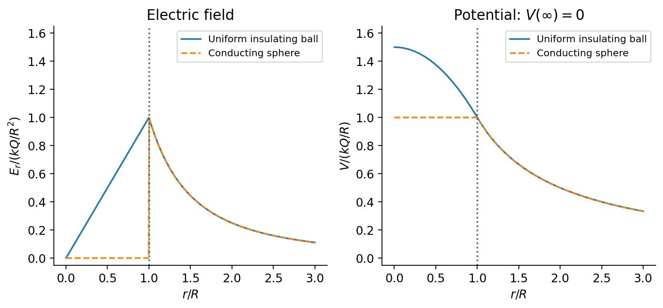
The conducting-sphere curve anticipates the equilibrium result developed in class 5. Both use the same \(Q\), \(R\), and zero at infinity.

9. From potential back to field

For an infinitesimal displacement,

\[ dV=-\mathbf E\cdot d\boldsymbol\ell =\frac{\partial V}{\partial x}dx+\frac{\partial V}{\partial y}dy+\frac{\partial V}{\partial z}dz. \]

Comparing independent coordinate displacements gives

\[ E_x=-\frac{\partial V}{\partial x},\qquad E_y=-\frac{\partial V}{\partial y},\qquad E_z=-\frac{\partial V}{\partial z},\qquad \mathbf E=-\nabla V. \]

Example: \(V=\alpha x^2-\beta y\) yields \(\mathbf E=(-2\alpha x,\beta,0)\). The gradient notation and its connection to divergence and curl are developed next.

10. Common errors

• Use \(\Delta U=q\Delta V\), including the sign of \(q\).
• Distinguish \(W_{\mathrm{field}}=-\Delta U\) from quasistatic \(W_{\mathrm{ext}}=\Delta U\).
• A zero potential is a reference-dependent value; a zero field is a statement about all spatial derivatives.
• An equipotential surface can have nonzero normal electric field.
• Sum each interaction pair once; omit point-charge self-interactions.
• Differentiate with respect to observation coordinates, not a source integration coordinate.
• Do not use \(V(\infty)=0\) for an ideal infinite line or infinite sheet.

References

Lecture 3 PDF pp. 3–16 gives work, potential, and equipotentials; pp. 17–22 covers charges, dipoles, and assembly energy; pp. 23–32 covers continuous sources and differentiation. Class 3, 13:09–96:44, adds the conservative-force/curl discussion. The uniformly charged ball is a class-4 worked example, approximately 24–29 minutes. The source map distinguishes these classroom supplements from slide-only material.