03_Newtonian Mechanics

1. Overview & Applicability

This section introduces the core focus of Newtonian mechanics and its physical limitations.

Core Relation: Newtonian mechanics primarily studies the relationship between force and acceleration.
Applicability (Limits of Newtonian Physics):
- Speed: It only applies at low speeds (\(v \ll c\)); at speeds approaching the speed of light, we must use Relativity.
- Scale: It only applies at the macroscopic scale; at the atomic or subatomic level, we must use Quantum Mechanics.

2. Newton's Three Laws of Motion

Newton's First Law (Law of Inertia):
- Definition: No force means no velocity change (which means no acceleration).
- Types of Force:
  - Contact force: Arises from physical contact.
  - Field force: Acts over a distance (e.g., gravity, electromagnetism).
Newton's Second Law:
- Equation:
  
  \[ \vec{F} = m\vec{a} \]
- where \(m = \text{mass}\).
Newton's Third Law:
- Equation:
  
  \[ \vec{F}_{12} = -\vec{F}_{21} \]
- Action and reaction forces are equal in magnitude and opposite in direction.

3. Reference Frames & Relative Motion

Inertial Reference Frame:
- Definition: A frame of reference where Newton's Laws strictly hold true.
Non-Inertial Frame:
- Example: An accelerating car (with acceleration \(\vec{a}\)).
Relative Motion & Observers:
- Projectile motion viewed from a frame moving horizontally with the same initial velocity \(\vec{v}_0\) simply looks like free fall (straight down).
- Different Inertial Observers:
  - Will agree on acceleration (\(\vec{a}\)).
  - Will disagree on position (\(\vec{x}\)) and velocity (\(\vec{v}\)).

4. Galilean Transformation

This part mathematically links the observations between a stationary frame and a frame moving at a constant velocity.

Assume a frame is moving at a constant velocity \(\vec{v}_0\) relative to a stationary frame. The displacement between their origins is \(\vec{v}_0t\).
Position Transformation:

\[ \vec{r}' = \vec{r} - \vec{v}_0t \]
Velocity Transformation: Taking the time derivative of the position equation:

\[ \Rightarrow \frac{d\vec{r}'}{dt} = \frac{d\vec{r}}{dt} - \vec{v}_0 \]

\[ \Rightarrow \vec{v}' = \vec{v} - \vec{v}_0 \]
Acceleration Transformation: Taking the time derivative of the velocity equation (since \(\vec{v}_0\) is constant, its derivative is zero):

\[ \Rightarrow \frac{d\vec{v}'}{dt} = \frac{d\vec{v}}{dt} \]

\[ \Rightarrow \vec{a}' = \vec{a} \]

(This proves that acceleration is the same in all inertial reference frames).

5. Analytical Tools

Free-Body Diagram (受力分析图)
Fictitious Force:
- A mathematical "correction" force used when analyzing motion inside a non-inertial (accelerating) reference frame so that Newton's Laws can still appear to be applied.
- Equation:
  
  \[ F_{\text{fictitious}} = -m\vec{a} \]
  
  (pointing in the opposite direction of the frame's acceleration).

6. Drag (Fluid Resistance)

This section outlines the two primary models for fluid resistance (drag) depending on the object's speed.

General Notes:
- \(\vec{v}\) represents the relative speed between the object and the fluid.
- \(\rho\) is the fluid density.
- \(A\) is the cross-sectional area of the object perpendicular to the motion.
Low-Speed Drag Model (Linear):
- Valid for low speeds or highly viscous fluids.
- Equation:
  
  \[ \vec{R} = -b\vec{v} \]
- (where \(b\) is a proportionality constant dependent on the object's shape and fluid properties).
High-Speed Drag Model (Quadratic):
- Valid for higher speeds (where air/fluid turbulence becomes a factor).
- Equation:
  
  \[ \vec{R} = -\frac{1}{2} C \rho A v^2 \hat{v} \]
- (where \(C\) is the drag coefficient, and \(\hat{v} = \frac{\vec{v}}{|\vec{v}|}\) is the unit vector representing direction).

6.1 "Free" Fall with Low-Speed Drag

This section analyzes an object falling under gravity while experiencing linear drag.

Setup & Differential Equation:
- FBD Components: Upward drag \(\vec{R} = -b\vec{v}\), downward gravity \(m\vec{g}\).
- Applying Newton's 2nd Law:
  
  \[ mg - bv = ma \Rightarrow mg - bv = m\frac{dv}{dt} \]
Definitions:
- Terminal Speed (\(v_t\)): The maximum constant speed reached when drag balances gravity (acceleration becomes zero).
  
  \[ v_t = \frac{mg}{b} \]
- Characteristic Time (\(\tau\)): The time constant of the system.
  
  \[ \tau = \frac{m}{b} = \frac{v_t}{g} \]
Kinematic Solutions:
- Velocity: Solving the differential equation yields:
  
  \[ v(t) = \frac{mg}{b}\left(1 - e^{-\frac{b}{m}t}\right) \Rightarrow v(t) = v_t(1 - e^{-t/\tau}) \]
- At \(t = \tau\): The speed reaches \(v = v_t(1 - e^{-1}) \approx 0.63 v_t\).
- Acceleration: Taking the time derivative of velocity:
  
  \[ a(t) = \frac{dv}{dt} = \frac{mg}{b} \cdot \frac{b}{m} e^{-\frac{b}{m}t} = g e^{-\frac{b}{m}t} \]

6.2 "Free" Fall with High-Speed Drag

This section evaluates the non-linear case where drag is proportional to velocity squared.

Terminal Speed Evaluation:
- At terminal velocity, acceleration is zero: \(mg = \frac{1}{2} C \rho A v_t^2\)
- \[\Rightarrow v_t = \sqrt{\frac{2mg}{C \rho A}}\]
True Time-Dependent Evaluation:
- Differential equation: \(mg - \frac{1}{2} C \rho A v^2 = m\frac{dv}{dt}\)
- Solving this non-linear ODE yields a hyperbolic tangent function:
  
  \[ v(t) = \sqrt{\frac{2mg}{C \rho A}} \tanh\left(\sqrt{\frac{g C \rho A}{2m}} t\right) \]
Question: How does terminal speed (\(v_t\)) scale with the size of an object?
- Mass is proportional to volume (radius cubed): \(m \propto r^3\)
- Cross-sectional area is proportional to radius squared: \(A \propto r^2\)
- Substituting these into the terminal speed formula:
  
  \[ v_t \propto \sqrt{\frac{r^3}{r^2}} \Rightarrow v_t \propto \sqrt{r} \]
- Conclusion: Larger objects have a higher terminal velocity.

7. Frictional Force

This section covers the mechanics of dry friction between solid surfaces.

Graph Analysis (\(|\vec{f}|\) vs \(|\vec{F}|\)):
- The friction force increases linearly to match the applied force until it reaches a breaking point (\(f_{s,\max}\)).
- Once motion begins, the friction force drops slightly and remains constant at the kinetic friction level (\(f_k\)).
Equations & Coefficients:
- Static Friction (\(f_s\)): Prevents motion. Maximum value is \(f_{s,\max} = \mu_s F_N\).
- Kinetic Friction (\(f_k\)): Opposes ongoing motion. \(f_k = \mu_k F_N\).
- \(\mu_s\): Coefficient of static friction.
- \(\mu_k\): Coefficient of kinetic friction (typically \(\mu_k < \mu_s\)).

7.1 Example: Static Friction

Problem Setup: A rope is wrapped around a pipe for one full circle (\(2\pi\)), hangs down holding an object of mass \(m\), and is pulled horizontally.
Contact Angle: The total angle the rope wraps around the pipe is \(\theta = 2\pi + \frac{\pi}{2} = \frac{5\pi}{2}\) radians. (Note: Changed "contact area" to the physically accurate term "contact angle").
Question: What is the range of horizontal force \(F\) required to keep the system in equilibrium (stationary)?
Lower Limit Derivation (When the mass is about to fall):
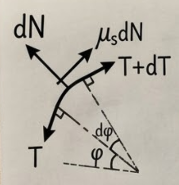
- Setup: Consider an infinitesimally small segment of the rope over an angle \(d\varphi\). The tension on one side is \(T\), and on the other is \(T+dT\). The normal force is \(dN\), and the friction opposing the impending slip is \(\mu_s dN\).
- Radial Force Balance:
  
  \[ dN = T\sin\frac{d\varphi}{2} + (T+dT)\sin\frac{d\varphi}{2} \]
  
  Applying the small-angle approximation (\(\sin \theta \approx \theta\)):
  
  \[ \Rightarrow dN = T d\varphi \]
- Tangential Force Balance:
  
  \[ (T+dT)\cos\frac{d\varphi}{2} + \mu_s dN = T\cos\frac{d\varphi}{2} \]
  
  Applying the small-angle approximation (\(\cos \theta \approx 1\)):
  
  \[ \Rightarrow dT + \mu_s dN = 0 \]
- Solving the Differential Equation:
  
  Substituting \(dN\) into the tangential equation gives:
  
  \[ \frac{dT}{T} = -\mu_s d\varphi \]
  
  Integrating both sides from the weight \(mg\) to the applied force \(F\), and from angle \(0\) to \(\frac{5\pi}{2}\):
  
  \[ \ln T \Big|_{mg}^F = -\mu_s \varphi \Big|_0^{5\pi/2} \]
  
  \[ \Rightarrow F = mg e^{-\frac{5\pi}{2}\mu_s} \]
Upper Limit Derivation (When the mass is about to be pulled up):
- The friction vector reverses direction to oppose the upward pull.
- This changes the sign in the integration, resulting in \(F = mg e^{+\frac{5\pi}{2}\mu_s}\) (where \(F > mg\)).
Conclusion:

\[ mg e^{-\frac{5\pi}{2}\mu_s} \le F \le mg e^{\frac{5\pi}{2}\mu_s} \]

7.2 Example: Kinetic Friction

This section calculates the final velocity of a particle traversing a semi-circular track with friction.

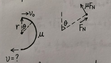
Setup: A particle enters a semi-circular track of radius \(r\) with initial velocity \(v_0\). The coefficient of kinetic friction is \(\mu\). What is the final velocity \(v_f\)?
Equations of Motion:
- The normal force provides the centripetal acceleration: \(F_N = m\frac{v^2}{r}\).
- Kinetic friction opposes motion: \(-\mu F_N = m\frac{dv}{dt}\).
Integration:

Substituting \(F_N\) into the friction equation:

\[ \Rightarrow -\mu \frac{v^2}{r} = \frac{dv}{dt} \]

Rearranging to separate variables (and utilizing the trick that \(v dt\) equals the infinitesimal distance \(ds\)):

\[ \Rightarrow -\frac{\mu}{r} (v dt) = \frac{dv}{v} \]

Integrating both sides. The integral of \(v dt\) is the total arc length of the semi-circle (\(\pi r\)):

\[ -\frac{\mu}{r} \int_{t_0}^{t_f} v dt = \int_{v_0}^{v_f} \frac{dv}{v} \]

\[ \Rightarrow -\frac{\mu}{r} \cdot (\pi r) = \ln v_f - \ln v_0 \]

\[ \Rightarrow v_f = v_0 e^{-\pi\mu} \]

8. Numerical Integration Methods

Solving a general problem: Given \(\vec{F}(\vec{r}, \vec{v}, t)\), solve for \(\vec{r}(t)\).

8.1 Euler Integration

An iterative method to approximate the state of a system at discrete time steps \(t_n = t_{n-1} + \Delta t\).

Step 0 (Initial State): * Time: \(t_0\)
- Position: \(\vec{r}_0\)
- Velocity: \(\vec{v}_0\)
- Acceleration: \(\vec{a}_0 = \vec{F}(\vec{r}_0, \vec{v}_0, t_0)/m\)
Step 1:
- \(t_1 = t_0 + \Delta t\)
- \(\vec{r}_1 = \vec{r}_0 + \vec{v}_0\Delta t\)
- \(\vec{v}_1 = \vec{v}_0 + \vec{a}_0\Delta t\)
- \(\vec{a}_1 = \vec{F}(\vec{r}_1, \vec{v}_1, t_1)/m\)
Step n:
- \(t_n = t_{n-1} + \Delta t\)
- \(\vec{r}_n = \vec{r}_{n-1} + \vec{v}_{n-1}\Delta t\)
- \(\vec{v}_n = \vec{v}_{n-1} + \vec{a}_{n-1}\Delta t\)
- \(\vec{a}_n = \vec{F}(\vec{r}_n, \vec{v}_n, t_n)/m\)

Error and Convergence:

The position error for Euler integration is on the order of \(O(\Delta t^2)\).
Convergence Check: Halve the time step repeatedly (\(\Delta t' = \frac{1}{2}\Delta t, \frac{1}{4}\Delta t, \dots\)) to verify numerical stability.

8.2 Verlet Integration

A more accurate integration scheme that does not explicitly require velocity for position updates after the first step.

\[ \vec{r}_{n+1} = 2\vec{r}_n - \vec{r}_{n-1} + \vec{a}_n \Delta t^2 \]

Proof (using Taylor expansion):

Let \(\vec{b} \equiv \frac{d\vec{a}}{dt}\). Expanding forward and backward in time:

\[ \vec{r}_{n+1} - \vec{r}_n = \vec{v}_n \Delta t + \frac{1}{2}\vec{a}_n \Delta t^2 + \frac{1}{6}\vec{b}_n \Delta t^3 + O(\Delta t^4) \]

\[ \vec{r}_{n-1} - \vec{r}_n = -\vec{v}_n \Delta t + \frac{1}{2}\vec{a}_n \Delta t^2 - \frac{1}{6}\vec{b}_n \Delta t^3 + O(\Delta t^4) \]

Adding these two equations cancels out the \(\vec{v}_n\) and \(\vec{b}_n\) terms, yielding the Verlet formula.

Key Notes on Verlet Integration:

Error: The position error is significantly reduced to \(O(\Delta t^4)\).
Initialization: \(\vec{r}_1\) is required to start the iteration, which can be approximated as:

\[ \vec{r}_1 \approx \vec{r}_0 + \vec{v}_0 \Delta t + \frac{1}{2}\vec{a}_0 \Delta t^2 \quad (O(\Delta t^3) \text{ error}) \]
Velocity \(\vec{v}_n\) is not required for calculating steps \(n > 1\).

8.3 Velocity Verlet Integration

Assumes the force \(\vec{F}(\vec{r}, t)\) has no dependence on velocity \(\vec{v}\). This method allows for simultaneous updating of both position and velocity.

\(\vec{r}_{n+1} = \vec{r}_n + \vec{v}_n \Delta t + \frac{1}{2}\vec{a}_n \Delta t^2\)
\(\vec{a}_{n+1} = \vec{F}(\vec{r}_{n+1}, t_{n+1})/m\)
\(\vec{v}_{n+1} = \vec{v}_n + \frac{1}{2}(\vec{a}_n + \vec{a}_{n+1})\Delta t\)
Error: \(O(\Delta t^4)\).
Advantage: It only depends on the immediately preceding step.

Compact Operator Form of Velocity Verlet:

Define operators for updating velocity (\(U_F\)) and position (\(U_v\)):

\[ U_F(\Delta t) \begin{pmatrix} \vec{r} \\ \vec{v} \end{pmatrix} = \begin{pmatrix} \vec{r} \\ \vec{v} + \vec{a}\Delta t \end{pmatrix} \]

\[ U_v(\Delta t) \begin{pmatrix} \vec{r} \\ \vec{v} \end{pmatrix} = \begin{pmatrix} \vec{r} + \vec{v}\Delta t \\ \vec{v} \end{pmatrix} \]

The full step can be written as a symmetric application of these operators:

\[ U_F\left(\frac{1}{2}\Delta t\right) U_v(\Delta t) U_F\left(\frac{1}{2}\Delta t\right) \begin{pmatrix} \vec{r}_n \\ \vec{v}_n \end{pmatrix} \]

Applying sequentially from right to left:

\[U_F\left(\frac{1}{2}\Delta t\right) \rightarrow \text{updates } \vec{v}_n \text{ to } \vec{v}_n' = \vec{v}_n + \frac{1}{2}\vec{a}_n\Delta t\]
\[U_v(\Delta t) \rightarrow \text{updates } \vec{r}_n \text{ to } \vec{r}_{n+1} = \vec{r}_n + \left(\vec{v}_n + \frac{1}{2}\vec{a}_n\Delta t\right)\Delta t\]

With \(\vec{r}_{n+1}\) calculated, the new acceleration \(\vec{a}_{n+1}\) can now be evaluated.
\[U_F\left(\frac{1}{2}\Delta t\right) \rightarrow \text{updates } \vec{v}_n' \text{ to } \vec{v}_{n+1} = \vec{v}_n + \frac{1}{2}\vec{a}_n\Delta t + \frac{1}{2}\vec{a}_{n+1}\Delta t\]