01_Rotation

1. Introduction: From Point Particle to Rigid Object

When transitioning from point mechanics, we introduce the extended rigid object—a non-deformable body. This introduces a new degree of freedom: Rotation.

Focus: Rotation of a rigid body about a fixed axis.

Angular Motion Definitions (Polar Coordinates)

In the plane perpendicular to the rotation axis, we use polar coordinates $(r, \theta)$. The arc length is $s = r\theta$.

Angular Displacement:

\[ \Delta\theta = \theta_f - \theta_i \]
Average Angular Speed:

\[ \omega_{ave} = \frac{\Delta\theta}{\Delta t} \]
Instantaneous Angular Speed:

\[ \omega \equiv \lim_{\Delta t \to 0} \frac{\Delta\theta}{\Delta t} = \frac{d\theta}{dt} \]
- Unit: $\text{rad/s}$ or $\text{s}^{-1}$
- Direction: " $+$ " is defined for counter-clockwise rotation.
Average Angular Acceleration:

\[ \alpha_{ave} \equiv \frac{\Delta\omega}{\Delta t} \]
Instantaneous Angular Acceleration:

\[ \alpha \equiv \lim_{\Delta t \to 0} \frac{\Delta\omega}{\Delta t} = \frac{d\omega}{dt} \]

2. Rotational Kinematics

Direction of Angular Velocity

The direction of $\vec{\omega}$ is determined by the Right-Hand Rule. If the fingers of your right hand curl in the direction of the rotation, your thumb points in the direction of the vector $\vec{\omega}$.

\[ \vec{\omega} = \omega \hat{w} \]

Constant Angular Acceleration

The kinematic equations for rotational motion with constant $\alpha$ perfectly mirror linear motion with constant $a$:

Rotation	Linear Motion
$\omega_f = \omega_i + \alpha t$	$v_f = v_i + at$
$\theta_f = \theta_i + \omega_i t + \frac{1}{2}\alpha t^2$	$x_f = x_i + v_i t + \frac{1}{2}at^2$
$\theta_f - \theta_i = \frac{\omega_f^2 - \omega_i^2}{2\alpha}$	$x_f - x_i = \frac{v_f^2 - v_i^2}{2a}$

Analogy Mapping: $x \leftrightarrow \theta$, $v \leftrightarrow \omega$, $a \leftrightarrow \alpha$.

Relation Between Linear and Angular Variables

Velocity:

\[ v = \frac{ds}{dt} = \frac{d(r\theta)}{dt} = r \frac{d\theta}{dt} = \omega r \]

Vector Form: $\vec{v} = \vec{\omega} \times \vec{r}$
Acceleration ($\vec{a} = \vec{a}_t + \vec{a}_r$):
- Tangential: $a_t = \frac{dv}{dt} = r \frac{d\omega}{dt} = \alpha r$
- Radial (Centripetal): $a_r = \frac{v^2}{r} = \omega^2 r$
- Total Magnitude: $a = \sqrt{a_t^2 + a_r^2} = \sqrt{\alpha^2 r^2 + \omega^4 r^2} = r \sqrt{\alpha^2 + \omega^4}$

3. Torque and Moment of Inertia

Torque ($\tau$)

Torque is the rotational analog of force. It is defined only when a reference axis is defined.

\[ \tau = (F \sin\phi) r = F d \]

图示：GP Rotation1

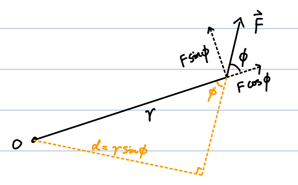
schematic diagram from the hand-written notes of Mr. ztWang

Where $d = r \sin\phi$ is the moment arm.

Total Torque from Multiple Forces: $\tau_{total} = \sum \tau_i$
Vector Form: $\vec{\tau} = \vec{r} \times \vec{F}$

Moment of Inertia ($I$) and Newton's Second Law for Rotation

For a point particle:

\[ F_t = m a_t \implies \tau = F_t r = m a_t r = (mr^2) \alpha \]

Defining the Moment of Inertia as $I \equiv mr^2$, we get the rotational analog of $F=ma$:

\[ \tau = I\alpha \]

Generalizing to a Rigid Body:

\[ dF_t = a_t dm \implies d\tau = r dF_t = r a_t dm = r^2 \alpha dm \]

\[ \tau_{total} = \int d\tau = \left(\int r^2 dm\right) \alpha \]

Defining $I = \int r^2 dm$, we conclude:

\[ \tau_{total} = I \alpha \]

Notes on Rigid Body Angular Motion:

$\vec{\omega}$ and $\vec{\alpha}$ are the same at any point on the rigid body, whereas $\vec{v}$ and $\vec{a}$ can vary by location.

The set $\{\vec{\tau}_{total}, \vec{\omega}, \vec{\alpha}\}$ fully characterizes the angular motion of a rigid body.

4. Energy, Work, and Power in Rotation

Rotational Kinetic Energy

\[ K_R = \int dK = \int \frac{1}{2}v^2 dm = \int \frac{1}{2}\omega^2 r^2 dm = \frac{1}{2}\omega^2 \int r^2 dm = \frac{1}{2}I\omega^2 \]

For a fixed axis, $K_R$ is the regular total kinetic energy.
If the axis is moving (e.g., rolling), $K_R$ is only the "rotational" component of the total kinetic energy.

Work and Power

Work:

\[ dW = \vec{F} \cdot d\vec{s} = (F_t)(r d\theta) = \tau d\theta \]

Vector form: $dW = \vec{\tau} \cdot d\vec{\theta}$ (Note: the radial force component $F_r$ does no work).
Instantaneous Power:

\[ P = \frac{dW}{dt} = \frac{\tau d\theta}{dt} = \tau \omega \]

Work-Kinetic Energy Theorem

Starting from $\tau_{total} = I\alpha$:

\[ \tau_{total} = I \frac{d\omega}{dt} \implies \tau_{total} d\theta = I \frac{d\omega}{dt} d\theta = I \omega d\omega \]

Integrating both sides:

\[ W_{total} = \int_{\theta_i}^{\theta_f} \tau_{total} d\theta = \int_{\omega_i}^{\omega_f} I \omega d\omega = \frac{1}{2}I\omega_f^2 - \frac{1}{2}I\omega_i^2 \]

5. Summary of Analogies: Linear vs. Rotational

Concept	Rotation	Linear Motion
Velocity	$\omega = d\theta/dt$	$v = dx/dt$
Acceleration	$\alpha = d\omega/dt$	$a = dv/dt$
Inertia	$I$ (Depends on axis)	$m$ (Intrinsic property)
Force / Torque	$\tau_{total} = I\alpha$	$F = ma$
Work	$W = \int_{\theta_i}^{\theta_f} \tau d\theta$	$W = \int_{x_i}^{x_f} F dx$
Kinetic Energy	$K_R = \frac{1}{2}I\omega^2$	$K = \frac{1}{2}mv^2$
Power	$P = \tau\omega$	$P = Fv$
Work-Energy	$W = K_{R,f} - K_{R,i}$	$W = K_f - K_i$

6. Calculating Moment of Inertia ($I$)

Example 1: Discrete Point Masses

图示：GP Rotation2

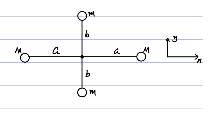
Four masses on a cross structure (masses $M$ at distance $a$ on x-axis; masses $m$ at distance $b$ on y-axis):

Axis $\parallel \hat{y}$: $I = Ma^2 + Ma^2 = 2Ma^2$
Axis $\parallel \hat{x}$: $I = mb^2 + mb^2 = 2mb^2$
Axis $\parallel \hat{z}$: $I = 2Ma^2 + 2mb^2$

Example 2: Uniform Rod

Mass $M$, length $L$. Linear mass density $\lambda = M/L$.

Axis through center:

\[ I = \int_{-L/2}^{L/2} x^2 (\lambda dx) = \lambda \left[ \frac{1}{3}x^3 \right]_{-L/2}^{L/2} = \frac{1}{12}ML^2 \]
Axis at one end:

\[ I = \int_{0}^{L} x^2 (\lambda dx) = \lambda \left[ \frac{1}{3}x^3 \right]_{0}^{L} = \frac{1}{3}ML^2 \]

Example 3: Spherical Shell (Axis through center)

图示：GP Rotation3

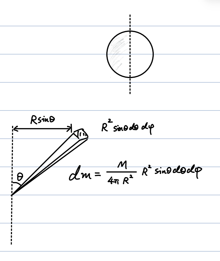
Mass $M$, Radius $R$. Area density $\sigma = \frac{M}{4\pi R^2}$.

Using spherical coordinates where $dm = \sigma (R^2 \sin\theta d\theta d\phi)$:

\[ I = \int r^2 dm = \frac{M}{4\pi} \int_{0}^{2\pi} d\phi \int_{0}^{\pi} (R\sin\theta)^2 \sin\theta d\theta \]

\[ I = \frac{M}{4\pi} (2\pi R^2) \int_{1}^{-1} (1 - \cos^2\theta) d(\cos\theta) = \frac{M R^2}{2} \left[ y - \frac{1}{3}y^3 \right]_{-1}^{1} = \frac{2}{3}MR^2 \]

Other Common Rigid Bodies (Proofs Omitted)

Solid Spherical Ball: $I = \frac{2}{5}MR^2$
Cylindrical Shell: $I = MR^2$
Solid Cylinder: $I = \frac{1}{2}MR^2$
Rectangular Plate (Axis through center, perpendicular to plate sides $a,b$): $I = \frac{1}{12}M(a^2 + b^2)$

7. Parallel Axis Theorem

Theorem:

\[ I = I_{cm} + Mh^2 \]

Where $I_{cm}$ is the moment of inertia through the Center of Mass (CM), and $h$ is the perpendicular displacement of the new axis from the CM axis.

Proof:

\[ I = \sum m_i r_i^2 = \sum m_i (\vec{r}_i' + \vec{h})^2 \]

\[ I = \sum m_i (r_i'^2 + 2\vec{r}_i'\cdot\vec{h} + h^2) = \sum m_i r_i'^2 + \left(\sum m_i\right)h^2 + 2\left(\sum m_i\vec{r}_i'\right)\cdot\vec{h} \]

Since the origin of $\vec{r}_i'$ is the CM, $\sum m_i\vec{r}_i' = 0$. This leaves:

\[ I = I_{cm} + M + 0 = I_{cm} + Mh^2 \]

Applications of Parallel Axis Theorem

Uniform Rod (axis at end): $I_{end} = I_{cm} + M\left(\frac{L}{2}\right)^2 = \frac{1}{12}ML^2 + \frac{1}{4}ML^2 = \frac{1}{3}ML^2$
Spherical Shell (axis on edge): $I_{edge} = I_{cm} + MR^2 = \frac{2}{3}MR^2 + MR^2 = \frac{5}{3}MR^2$
Spherical Shell (far-away axis $h \gg R$): $I_{far} = I_{cm} + Mh^2 = M\left(h^2 + \frac{2}{3}R^2\right) \approx Mh^2$ (Acts like a point particle).

8. Comprehensive Example: The Rotating Rod

Scenario: A uniform rod of mass $M$ and length $L$ is pivoted at its left end. It is released from a horizontal position.

图示：GP Rotation4

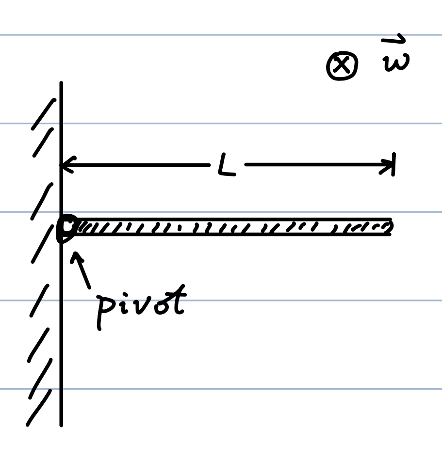
Questions: What is the initial angular acceleration $\alpha$? What is the initial linear acceleration of the right end?

Solution:

Find Total Torque:
```
Integrate the torque of infinitesimal mass elements along the rod due to gravity ($g$).

$$
```
\tau_{total} = \int_{0}^{L} \left(\frac{M}{L}dx\right) \cdot g \cdot x = \frac{Mg}{L} \left[ \frac{1}{2}x^2 \right]_{0}^{L} = \frac{1}{2}MgL $$
Find Angular Acceleration:
```
Using $I = \frac{1}{3}ML^2$ for a rod pivoted at its end:

$$
```
\tau_{total} = I\alpha \implies \alpha = \frac{\tau_{total}}{I} = \frac{\frac{1}{2}MgL}{\frac{1}{3}ML^2} = \frac{3}{2}\frac{g}{L} $$
Find Linear Acceleration at the Right End:

\[ a_t = \alpha L = \left(\frac{3}{2}\frac{g}{L}\right) L = \frac{3}{2}g \]

(Notice that the far end of the rod accelerates faster than gravity initially!)

Rotation	Linear Motion
\(\omega_f = \omega_i + \alpha t\)	\(v_f = v_i + at\)
\(\theta_f = \theta_i + \omega_i t + \frac{1}{2}\alpha t^2\)	\(x_f = x_i + v_i t + \frac{1}{2}at^2\)
\(\theta_f - \theta_i = \frac{\omega_f^2 - \omega_i^2}{2\alpha}\)	\(x_f - x_i = \frac{v_f^2 - v_i^2}{2a}\)

Concept	Rotation	Linear Motion
Velocity	\(\omega = d\theta/dt\)	\(v = dx/dt\)
Acceleration	\(\alpha = d\omega/dt\)	\(a = dv/dt\)
Inertia	\(I\) (Depends on axis)	\(m\) (Intrinsic property)
Force / Torque	\(\tau_{total} = I\alpha\)	\(F = ma\)
Work	\(W = \int_{\theta_i}^{\theta_f} \tau d\theta\)	\(W = \int_{x_i}^{x_f} F dx\)
Kinetic Energy	\(K_R = \frac{1}{2}I\omega^2\)	\(K = \frac{1}{2}mv^2\)
Power	\(P = \tau\omega\)	\(P = Fv\)
Work-Energy	\(W = K_{R,f} - K_{R,i}\)	\(W = K_f - K_i\)