03_heat

1. Heat and Phase Transitions

• Heat Capacity: The heat capacity (\(C\)) dictates the temperature change (\(\Delta T\)) when heat (\(\Delta Q\)) is absorbed.

  \[ C = \frac{\Delta Q}{\Delta T} \implies \Delta T = \frac{\Delta Q}{C} \]

• Phase Transitions (Exception to \(\Delta T\)): When water undergoes a phase transition (e.g., melting at the freezing point \(T_F\) or boiling at the vaporizing point \(T_V\)), heat is absorbed but the temperature remains unchanged.

• Latent Heat: The heat required for a phase change is given by:

  \[ Q = LM \]

  (Where \(L\) is the heat of transformation and \(M\) is the mass).

  • Heat of Fusion (Ice to Water): \(L_F = 333 \text{ kJ/kg}\) \(\implies Q_F = L_F M\)

  • Heat of Vaporization (Water to Steam): \(L_V = 2256 \text{ kJ/kg}\) \(\implies Q_V = L_V M\)

• Units of Heat:

  • Specific heat of water: \(4184 \text{ J}\cdot\text{kg}^{-1}\cdot\text{K}^{-1} = 4.184 \text{ J}\cdot\text{g}^{-1}\cdot\text{K}^{-1}\)

  • Small calorie (gram-calorie): \(1 \text{ cal} \equiv 4.184 \text{ J}\)

  • Grand calorie (kilogram-calorie or food calorie): \(1 \text{ Cal} \equiv 4184 \text{ J}\)

    (Example: A 140 Cal soda can contains enough energy to raise the temperature of 1 kg of water by 140 K).

2. Heat Conduction

Heat transfer across a boundary translates microscopically to the transfer of molecular kinetic energy from a high-temperature region to a low-temperature region.

• Macroscopic View (Fourier's Law of Heat Conduction):

  \[ j_q \equiv \frac{dQ}{A dt} = -k \frac{dT}{dx} \]

  • \(j_q\): Heat current (heat per unit area per unit time).

  • \(A\): Cross-sectional area.

  • \(k\): Thermal conductivity (material-specific, e.g., \(k_{\text{metal}} \gg k_{\text{wood}}\)).

  • The negative sign indicates that the direction of heat flow (\(j_q\)) is opposite to the temperature gradient (\(\frac{dT}{dx}\)).

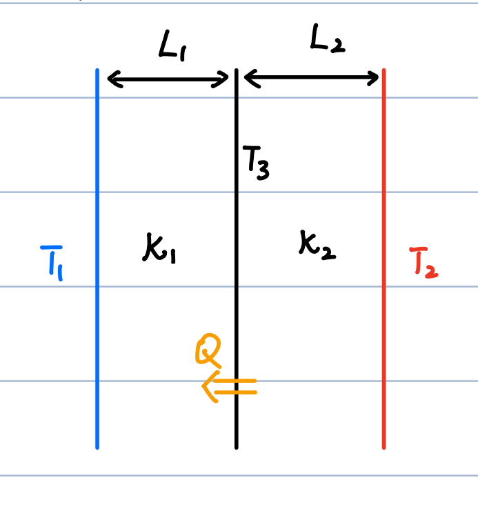
• Example Calculation (Two-Layer Slab): Given two adjacent materials with thicknesses \(L_1, L_2\) and conductivities \(k_1, k_2\), placed between outer temperatures \(T_1\) and \(T_2\), the interface temperature \(T_3\) and steady-state heat current are found by equating the heat flux through both layers:

  \[ j_q = -k_1 \frac{T_3 - T_1}{L_1} = -k_2 \frac{T_2 - T_3}{L_2} \]

  Solving this yields:

  \[ T_3 = \frac{k_1 T_1 / L_1 + k_2 T_2 / L_2}{k_1 / L_1 + k_2 / L_2} \quad \text{and} \quad j_q = - \frac{T_2 - T_1}{L_1/k_1 + L_2/k_2} \]

3. Mean Free Path (\(l\))

The mean free path is the average distance a molecule travels between collisions.

• Formula:

  \[ l = \frac{1}{\sqrt{2} \pi d^2 (N/V)} \]

  (Where \(d\) is the molecular diameter and \(N/V\) is the number density).

• Derivation Summary:

  • The volume swept by a molecule in time \(t\) is an effective "tube" of volume \(\pi d^2 \cdot \overline{v_r} t\), where \(\overline{v_r}\) is the relative average speed.

  • The number of collisions in this tube is \((N/V) \cdot \pi d^2 \overline{v_r} t\).

  • Mean free path \(l = \frac{\text{total distance}}{\text{number of collisions}} = \frac{\overline{v} t}{(N/V) \pi d^2 \overline{v_r} t} = \frac{\overline{v}/\overline{v_r}}{\pi d^2 N/V}\)

  • Using the Maxwell speed distribution and effective mass (\(m' = m/2\)), it is proven that \(\overline{v_r} = \sqrt{2} \overline{v}\). Substituting this confirms the formula.

• Alternative Form (Ideal Gas): Using \(pV = N k_B T\):

  \[ l = \frac{k_B T}{\sqrt{2} \pi d^2 p} \]

• Example (Air at 20°C):

  • Number density: \(N/V = \frac{p}{k_B T} = 2.50 \times 10^{25} \text{ m}^{-3}\)

  • Assuming \(d = 2 \times 10^{-10} \text{ m}\), the calculated mean free path is \(l = 2.25 \times 10^{-7} \text{ m}\).

  • This is much larger than the average molecular separation (\(\approx 3.4 \times 10^{-9} \text{ m}\)).

  • Collision frequency (\(f = \frac{\overline{v}}{l}\)) is approximately \(2 \times 10^9 \text{ s}^{-1}\).

4. Microscopic Derivation of Thermal Conductivity

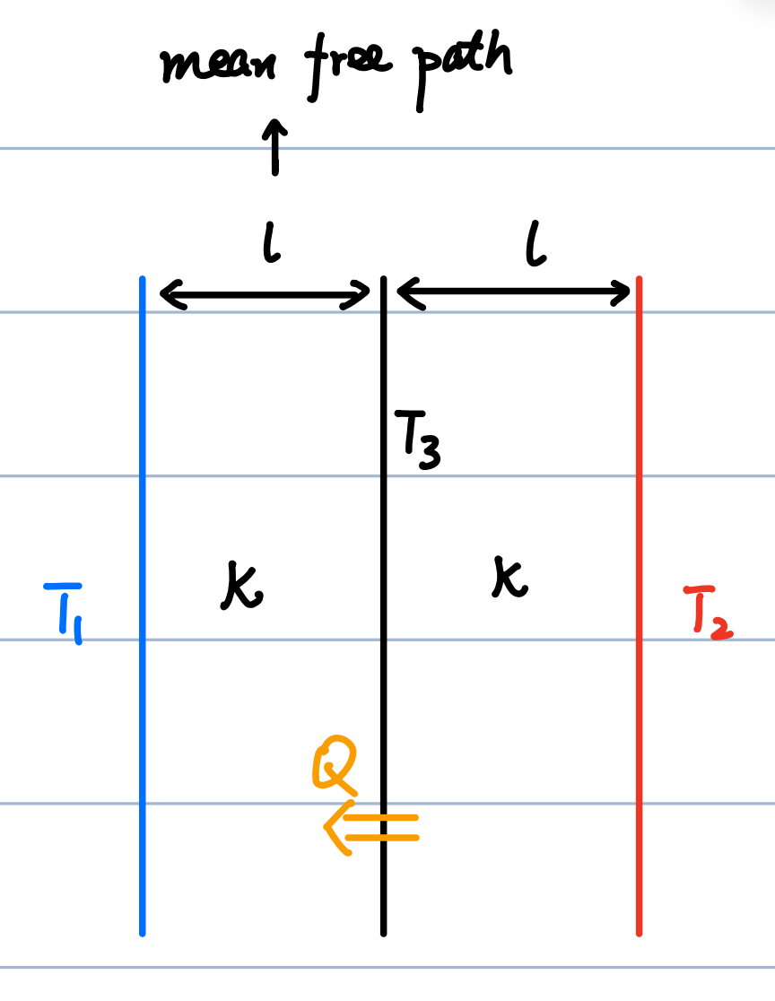
We can derive the macroscopic thermal conductivity (\(k\)) from microscopic kinetic theory by analyzing molecular exchange across an imaginary plane.

• Temperature Gradient Setup: Consider molecules exchanging between planes separated by a distance of \(l\) (mean free path).

  \[ \frac{dT}{dx} = \frac{T_2 - T_1}{2l} \]

• Heat Flux Expression:

  \[ \frac{dQ}{A dt} = N_{1 \rightarrow 2} \left( \frac{\text{DOF}}{2} k_B T_1 \right) - N_{1 \leftarrow 2} \left( \frac{\text{DOF}}{2} k_B T_2 \right) \]

  (Where DOF represents degrees of freedom \(t+r+2s\)).

• Particle Flux: Assuming 3D isotropic motion, 1/6th of particles move along any specific positive or negative axis direction.

  \[ N_{1 \rightarrow 2} \approx \frac{1}{6} \left(\frac{N}{V}\right)_1 \overline{v_1} \]

• Simplification: Assuming density and average speed vary minimally between the closely spaced planes \(\left(\left(\frac{N}{V}\right)_1 \overline{v_1} \approx \left(\frac{N}{V}\right)_2 \overline{v_2} \approx \frac{N}{V} \overline{v}\right)\):

  \[ \frac{dQ}{A dt} \approx \frac{1}{6} \frac{N}{V} \overline{v} \cdot \frac{\text{DOF}}{2} k_B (T_1 - T_2) \]

• Applying Specific Heat: Using \(C_V = \frac{\text{DOF}}{2} N k_B\), specific heat \(c_v = \frac{C_V}{M}\), and density \(\rho = \frac{M}{V}\):

  \[ j_q = \frac{1}{6} \frac{1}{V} \overline{v} C_V (T_1 - T_2) = \frac{1}{6} \rho \overline{v} c_v (T_1 - T_2) \]

• Final Thermal Conductivity (\(k\)): Equating the microscopic heat current to Fourier's law (\(j_q = -k \frac{dT}{dx}\)):

  \[ \frac{1}{6} \rho \overline{v} c_v (T_1 - T_2) = -k \frac{T_2 - T_1}{2l} \]
  \[ k = \frac{1}{3} \rho \overline{v} l c_v \]