02_gas

1. Kinetic Theory of Ideal Gases

Fundamental Assumptions

To model an ideal gas, the following assumptions are made regarding its molecules:

Negligible molecular volume: The volume of the molecules is infinitely small compared to the distance between them.
Short-range forces: Intermolecular forces are assumed to be zero except during collisions.
Elastic collisions: Collisions between molecules and with the container walls conserve kinetic energy.
Identical molecules: All molecules in the gas are perfectly identical.

Derivation of Pressure

Consider a cubic container of side length $L$. When a single molecule collides with the right-hand wall, its velocity in the x-direction reverses ($v_x \rightarrow -v_x$).

Momentum change: $\Delta p_x = (-m v_x) - m v_x = -2 m v_x$
Time interval between collisions: $\Delta t = \frac{2L}{v_x}$
Force from a single molecule: $F_x = \frac{|\Delta p_x|}{\Delta t} = \frac{2 m v_x}{2L / v_x} = \frac{m v_x^2}{L}$

To find the total pressure $P$ exerted by $N$ molecules, we sum the individual forces and divide by the area $L^2$:

\[ P = \frac{F_{x1} + F_{x2} + \dots + F_{xN}}{L^2} = \frac{m}{L^3} (v_{x1}^2 + v_{x2}^2 + \dots + v_{xN}^2) \]

Using the average squared velocity $\overline{v_x^2} \equiv \frac{1}{N} (v_{x1}^2 + \dots + v_{xN}^2)$ and substituting the number of moles $n = \frac{N}{N_A}$ (where $N_A$ is Avogadro's number):

\[ P = \frac{N m}{L^3} \overline{v_x^2} = \frac{n N_A m}{L^3} \overline{v_x^2} \]

Since velocity is isotropic, $v^2 = v_x^2 + v_y^2 + v_z^2 \Rightarrow \overline{v_x^2} = \frac{1}{3}\overline{v^2}$. Substituting this and $V = L^3$:

\[ P = \frac{n N_A m}{3V} \overline{v^2} \]

Comparing this result with the Ideal Gas Law ($PV = nRT$), we can solve for the root-mean-square (rms) speed:

\[ v_{rms} \equiv \sqrt{\overline{v^2}} = \sqrt{\frac{3RT}{N_A m}} = \sqrt{\frac{3k_B T}{m}} \]

2. Kinetic Energy & The Equipartition Theorem

Average Translational Kinetic Energy

Using the rms speed, the average translational kinetic energy per molecule is:

\[ K_{avg} = \frac{1}{2}m\overline{v^2} = \frac{1}{2}m v_{rms}^2 = \frac{3}{2} k_B T \]

Key Takeaway: Temperature is a direct macroscopic measure of molecular kinetic energy.

Equipartition Theorem

The average kinetic energy per degree of freedom is:

$\frac{1}{2}k_B T$ per molecule
$\frac{1}{2}RT$ per mole

For example, a monoatomic gas has 3 translational modes (x, y, z), so:

\[ \frac{1}{2}m\overline{v_x^2} = \frac{1}{2}m\overline{v_y^2} = \frac{1}{2}m\overline{v_z^2} = \frac{1}{2}k_B T \]

Internal Energy

For a monoatomic ideal gas, the total internal energy $U$ is simply the sum of all translational kinetic energy:

\[ U = \frac{3}{2} N k_B T = \frac{3}{2} n R T \]

3. Heat Capacity & Degrees of Freedom

Definitions

Heat capacity: $C \equiv \frac{\Delta Q}{\Delta T}$
Specific heat capacity (per mass): $c \equiv \frac{C}{M}$
Molar heat capacity (per mole): $C_m \equiv \frac{C}{n}$

Molar Heat Capacities ($C_V$ and $C_P$)

At constant volume ($C_V$): For a monoatomic gas, work is zero.

\[ C_V = \frac{1}{n}\left(\frac{dU}{dT}\right)_V = \frac{3}{2}R \]
At constant pressure ($C_P$): Work is done as the gas expands ($\Delta W = p \Delta V$).

\[ C_P = \frac{1}{n}\left(\frac{dU}{dT} + p\frac{dV}{dT}\right)_P \]

Since $pV = nRT \Rightarrow p\left(\frac{dV}{dT}\right)_P = nR$, we get Mayer's relation:

\[ C_P = C_V + R \]

Degrees of Freedom ($f$)

The number of degrees of freedom is calculated as $f = t + r + 2s$, where:

$t$: translational modes
$r$: rotational modes
$s$: oscillatory (vibrational) modes. (Note: Oscillation contributes $2s$ because it contains both kinetic energy $\frac{1}{2}RT$ and potential energy $\frac{1}{2}RT$).

Molecule Classifications:

N-atom linear molecule (e.g., $H_2$, $CO_2$): $t=3$, $r=2$, $s=3N-5$
N-atom nonlinear molecule (e.g., $H_2O$): $t=3$, $r=3$, $s=3N-6$

Example ($H_2$ Gas):

For $H_2$ ($N=2$), $t=3$, $r=2$, $s=3(2)-5=1 \Rightarrow f = 7$. Theoretically, $C_V = \frac{7}{2}R$.

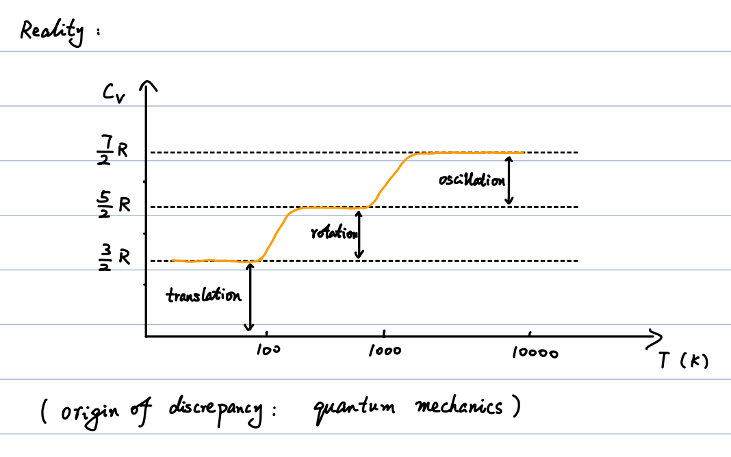
Reality Check (Quantum Mechanics): In reality, heat capacity depends on temperature because quantum mechanics dictates that energy levels are discrete.

At low temperatures (~100 K): Only translation is active ($C_V = \frac{3}{2}R$).
At room temperatures (~1000 K): Rotation unlocks ($C_V = \frac{5}{2}R$).
At extremely high temperatures (~10000 K): Oscillation unlocks ($C_V = \frac{7}{2}R$).

图示：General physics gas1

4. Statistical Mechanics & Probability Distributions

Basics of Probability Distribution

For a probability distribution function $f(v)$, the probability of finding a particle's velocity in the range $[v, v+dv]$ is $f(v)dv$.

Normalization: $\int_{-\infty}^{\infty} f(v)dv = 1$
Average velocity: $\overline{v} = \int_{-\infty}^{\infty} v f(v)dv$
Root-mean-square velocity: $v_{rms} = \sqrt{\int_{-\infty}^{\infty} v^2 f(v)dv}$

Maxwell Distribution of Velocity (1860)

In 3D space, assuming an isotropic distribution (no directional preference), the velocity vector distribution is:

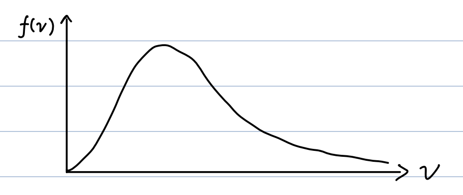
\[ f(\vec{v}) = f(v_x)f(v_y)f(v_z) = \left(\frac{m}{2\pi k_B T}\right)^{3/2} e^{-\frac{m v^2}{2k_B T}} \]

To convert this to a speed distribution (scalar $v$), we integrate over all angles ($\theta, \phi$) in spherical coordinates. The volume element becomes $4\pi v^2 dv$:

\[ f(v) = 4\pi \left(\frac{m}{2\pi k_B T}\right)^{3/2} e^{-\frac{m v^2}{2k_B T}} v^2 \]

图示：General physics gas2

Characteristic Speeds

By analyzing the speed distribution function $f(v)$, we can extract three specific speeds:

Most Probable Speed ($v_p$): Found by taking the derivative $\frac{df(v)}{dv} = 0$.
```
$$
```
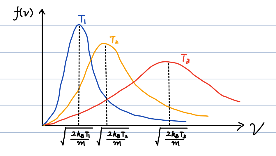
v_p = \sqrt{\frac{2 k_B T}{m}} $$
Average Speed ($\overline{v}$): Calculated via $\int_0^\infty v f(v)dv$.
```
$$
```
\overline{v} = \sqrt{\frac{8 k_B T}{\pi m}} \approx \sqrt{\frac{2.55 k_B T}{m}} $$
Root-Mean-Square Speed ($v_{rms}$): Calculated via $\sqrt{\int_0^\infty v^2 f(v)dv}$.

\[ v_{rms} = \sqrt{\frac{3 k_B T}{m}} \]

图示：General physics gas3

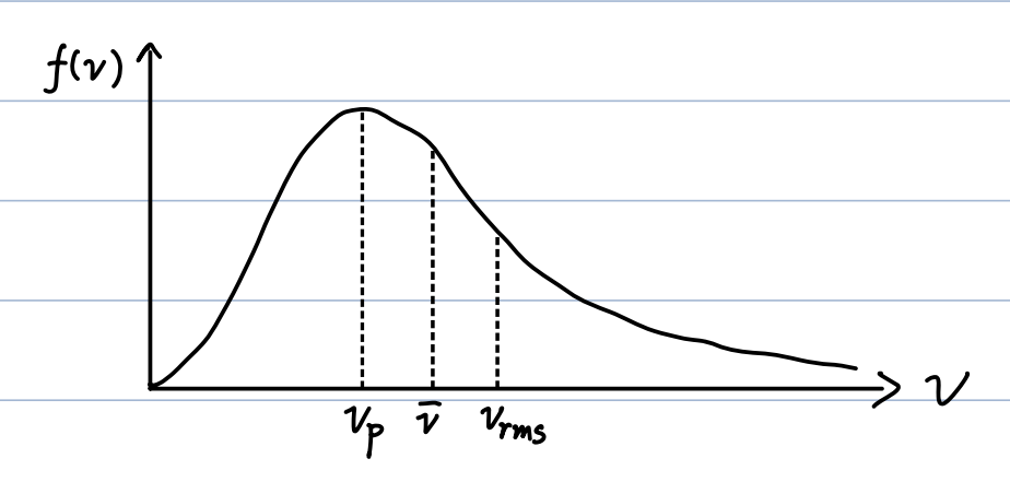
Order of magnitudes: $v_p < \overline{v} < v_{rms}$

Temperature Dependence

As temperature $T$ increases ($T_1 < T_2 < T_3$), the peak of the $f(v)$ curve shifts to the right (higher speeds) and the curve flattens and widens out.

图示：General physics gas4

5. Maxwell-Boltzmann Distribution

When an external potential energy field $\epsilon_p(\vec{r})$ is present, the distribution combines both spatial and momentum variables:

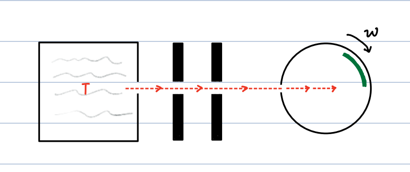
\[ f_{MB}(\vec{r}, \vec{v}) \propto e^{-\left[\frac{1}{2}m v^2 + \epsilon_p(\vec{r})\right] / k_B T} \]

Experimental Verification: The Maxwell distribution was experimentally verified by Otto Stern in 1920 using an oven emitting particles through slits toward a rotating cylindrical target. Particles with different speeds hit different angular positions on the target, perfectly mapping the theoretical speed distribution curve.

图示：General physics gas5