General Physics II · 普通物理学 II
First six classes: electrostatics, conductors, and the foundations of electric transport and capacitance. These notes combine the supplied lecture slides with the classroom explanations, derivations, and examples. English is the main language; Chinese annotations clarify terminology and difficult distinctions.
The semester introduction identifies Xin Lu as the instructor. The supplied slide decks credit Xin Lu / Gentaro Watanabe. The wider course includes magnetism, optics, and quantum physics; the notes below follow the actual progress of the first six classes.
Learning route(学习路线)
| Class | Notes | Main questions |
|---|---|---|
| 1 | Charge, Coulomb's law, and electric fields | What is charge? How do we define and visualize a field? What is a dipole? |
| 2 | Continuous charge and Gauss's law | How does a sum become an integral? When does symmetry determine the field? |
| 3 | Electric potential and potential energy | Why is electrostatic work path independent? How do scalar potentials simplify calculations? |
| 4 | The triangle of electrostatics | How are charge density, field, and potential related locally? What do divergence and curl mean? |
| 5 | Conductors, shielding, and image charges | How do mobile charges reach equilibrium? How do boundary conditions replace unknown charge distributions? |
| 6 | Current, resistance, and capacitance | How does microscopic motion produce current and resistance? How does geometry determine capacitance? |
- Mathematical toolkit: vectors, Taylor expansion, line/surface integrals, spherical coordinates, and point-charge distributions.
- Formula sheet and conceptual checks: formulas with their conditions, units, and common mistakes.
- Source map and scope: PDF page ranges, classroom timestamps, supplemental discussions, and editorial corrections.
- Figure provenance and reproduction: all figures are original mathematical diagrams or plots.
The central idea
We start with interactions between charges, then describe those interactions using fields and potentials. The same laws can be written as global integral statements or local differential equations. Conductors add boundary conditions; moving charges add conservation and transport laws.
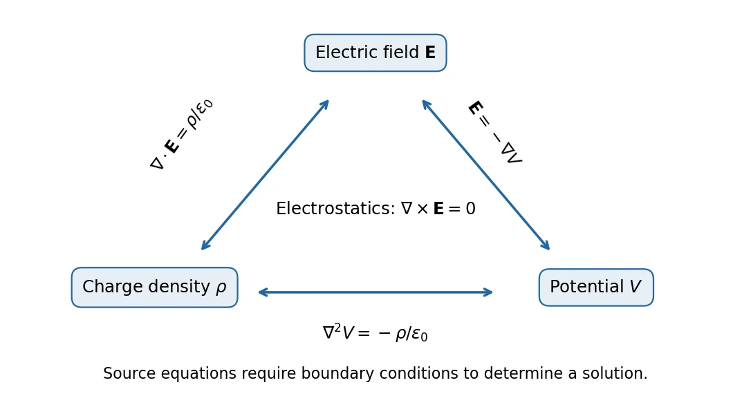
中文提示:前四课建立“电荷—电场—电势”的联系;第五课加入导体的边界条件;第六课开始研究电荷流动及元件的响应。公式之间的联系和适用条件,比孤立背诵更重要。
Prerequisites and notation
Prerequisites: Newtonian mechanics, work and energy, vector algebra, differentiation, elementary integration, and basic multivariable calculus. The mathematical toolkit supplies the conventions used here.
| Symbol | Meaning | SI unit |
|---|---|---|
| \(q,Q\) | Signed charge; total charge | C |
| \(\lambda,\sigma_s,\rho_q\) | Line, surface, and volume charge density | C/m, C/m², C/m³ |
| \(\mathbf E,V,U\) | Electric field, electric potential, potential energy | N/C = V/m, V, J |
| \(\mathbf p\) | Electric dipole moment, from negative to positive charge | C·m |
| \(i,\mathbf J\) | Signed current through an oriented surface; current density | A, A/m² |
| \(\rho_{\mathrm{res}},\sigma_{\mathrm{cond}}\) | Resistivity; conductivity | Ω·m, S/m |
| \(R,C\) | Resistance; capacitance | Ω, F |
We distinguish \(\rho_q\) from \(\rho_{\mathrm{res}}\), and \(\sigma_s\) from \(\sigma_{\mathrm{cond}}\): the original slides reuse \(\rho\) and \(\sigma\) for different physical quantities. Position is \(\mathbf r\), and \(r=|\mathbf r|\). The constant \(k=1/(4\pi\epsilon_0)\approx8.99\times10^9\ \mathrm{N\,m^2/C^2}\).
Unless stated otherwise, field calculations use vacuum, prescribed stationary sources, and ideal conductors in electrostatic equilibrium. Infinite sheets and lines are idealizations of finite systems observed sufficiently far from their edges or ends. A linear capacitor assumes fixed geometry and a fixed linear dielectric response; the first six classes primarily use vacuum examples.
How to work through a problem
- Specify the source, observation point, physical region, and boundary/reference conditions.
- Use symmetry to determine permitted field components before integrating.
- Choose Coulomb integration, Gauss's law, a potential integral, or a boundary-value construction.
- Keep signed charges and oriented normals explicit.
- Check dimensions, limiting cases, continuity or jumps at boundaries, and total charge.
The course introduction emphasizes understanding and independent reasoning. These notes remain marked draft: transcription errors have been corrected where the slides, calculations, and supporting references resolve them, but this is not a claim of exhaustive textbook review.
Course introduction record(课程导论记录)
The classroom introduction sketches electricity in weeks 1–4, magnetism in weeks 5–8, optics in weeks 9–12, and quantum physics in weeks 13–16. This is the introductory course outline, not a claim about the detailed schedule of future classes.
The introduction slide records tentative assessment weights of homework 30%, quizzes and midterm 30%, and final examination 40%. It also records roughly twelve problem sets and paper submission during the first Tuesday class. Current assignment instructions and any changes should be taken from the course announcements rather than inferred from this historical slide record.
The introductory reading list includes Halliday, Resnick, and Walker's Fundamentals of Physics, Feynman's Lectures on Physics, and the Berkeley electricity-and-magnetism text. Individual lecture PDFs additionally provide chapter references to Halliday, Resnick & Krane, and lecture 4 names Griffiths and Fleisch. The local slide decks remain the source of their particular edition/chapter conventions.
Coverage boundary
Capacitor series/parallel combinations and the semiconductor/superconductor discussion are included because they occur in class 6. Peltier and Hall effects and displacement current receive only the brief conceptual preview given in that class. Full circuit analysis, RC transients, capacitor energy density, dielectric theory, magnetic fields, optics, and quantum mechanics await later classes.