Introduction to Verilog HDL (*)

1. Background: Heterogeneous Computing

Modern computing utilizes various hardware architectures, each with distinct trade-offs.

Feature	CPU	GPU	FPGA (Field Programmable Gate Array)	ASIC (Application-Specific Integrated Circuit)
Compute Adaptability	High	Medium	Low	None
Compute Power	Medium	High	High	Medium
Latency	Medium	High	Low	Ultra low
Throughput	Low	High	High	High
Parallelism	Low	High	High	High
Power Efficiency	Medium	Low	Medium	High

Digital Circuit Design Focus: This course primarily focuses on design for FPGAs and ASICs.

2. Hardware Description Language (HDL)

• Definition: An HDL is a language that uses formal methods to describe digital circuits and design digital logic systems.

• Industry Standards: Verilog and VHDL are the dominant hardware description languages used in the industry.

3. HDL-Based Design Flow

The standard workflow for designing digital hardware using HDL consists of several sequential stages. While ASIC and FPGA flows are similar, they diverge at the physical design phase.

1. Logic Design with HDL: Writing the actual code.

   • Involves defining modules (module), ports (input, output), and internal logic using assignment statements (assign).

2. Simulation (Behavioral/Functional):

   • Verifying the logic using a Testbench.

   • A testbench provides input stimuli (using delays like #2) and monitors outputs (using $display) to ensure functional correctness without synthesizing hardware.

3. Synthesis: Translating the HDL code into hardware primitives.

   • Parsing: Checking syntax.

   • Multi-level synthesis: Note that not all HDL code is synthesizable (some is for simulation only).

   • Technology mapping: Mapping the logic to specific hardware library components.

4. Physical Design (Place & Route):

   • Placement: Deciding where components physically go on the chip.

   • Routing: Connecting the placed components.

   • Includes Static Timing Analysis (STA), LVS (Layout vs. Schematic), and DRC (Design Rule Checking).

   • Generating results:

     • ASIC: Generates a layout file.

     • FPGA: Generates a bitstream file.

5. Final Step:

   • ASIC: Tape-out (sending the design to a foundry for manufacturing). Wait time is typically 1-3 months.

   • FPGA: Downloading the bitstream file to configure the hardware instantly.

4. Verilog HDL: Lexical Conventions

Verilog syntax is heavily influenced by the C programming language.

Basic Rules

• Case-sensitive: Wire and wire are different.

• Keywords: All reserved keywords are in lowercase.

• Whitespace: Blank spaces (\b), tabs (\t), and newlines (\n) are generally ignored except in strings or when separating tokens.

• Comments: Identical to C.

Number Specifications

• Sized Numbers: <size>'<base><number>

  • <size>: Number of bits (in decimal).

  • <base>: Decimal (d/D), Binary (b/B), Octal (o/O), Hexadecimal (h/H).

  • Examples: 4'b1111, 12'habc, 16'd255.

• Unsized Numbers:

  • Default base is decimal. Default size is usually at least 32 bits (compiler dependent).

  • Examples: 23232, 'habc, 'o234.

• Negative Numbers: The minus sign must be placed before the size (e.g., -6'd3). 4'd-2 is illegal. Numbers are stored using Two's complement.

• Formatting: Underscores (_) can be used to improve readability (e.g., 12'b1111_0000_1010) but cannot be the first character.

Special Values: X, Z, and ?

• x: Unknown value.

• z: High-impedance value.

• ?: Acts as an alternative to z in numbers (e.g., 4'b10?? is the same as 4'b10zz).

• Extension Rules: If the specified size is larger than the value provided:

  • Padded with x if the MSB is x.

  • Padded with z if the MSB is z.

  • Zero-extended otherwise. (e.g., 6'hx becomes 6'bxx_xxxx).

Identifiers and Strings

• Strings: Enclosed in double quotes ("Hello World\n").

• Identifiers: Alphanumeric characters, _, and $. Must start with an alphabetical character or _. (Only system tasks start with $).

• Escaped Identifiers: Used for special naming conventions. Start with a backslash \ and end with whitespace. Can contain any printable character. (e.g., \a+b-c ).

5. Basic Syntax: Structure and Types

Modules and Instantiation

• Module Definition: The fundamental building block.

  module module_name (port_list);
      // Data type definition
      // Logic function description
  endmodule
  

• Instantiation: Placing a module inside another module.

  model_name instance_identifier (port_related_list);

Data Types

• Net (wire): Represents physical connections between structural entities. Does not store value.

• Register (reg): Represents a storage element. Holds its value until a new value is assigned.

• Vectors and Arrays:

  • Vector (multi-bit signal): wire [7:0] a;

  • Array: reg [15:0] mem [1023:0];

• Parameter: Defines local constants within a module scope.

Port Types

• input: Defined internally as a wire. Can be instantiated as a wire or reg in the higher-level module.

• output: Can be defined internally as a wire or reg. Must be instantiated as a wire in the higher-level module.

6. Operators and Precedence

Operators are listed below from Highest to Lowest Precedence:

1. Unary: + - ! ~

2. Multiply, Divide, Modulus: * / %

3. Add, Subtract: + -

4. Shift: << >>

5. Relational: < <= > >=

6. Equality: == != === !==

7. Bitwise Operation: & > ^ > |

8. Logical: && > ||

9. Conditional (Ternary): ? :

7. Modeling Methods

Verilog supports varying levels of abstraction for describing hardware.

Implementation of a Two-Bit Greater-Than Comparator (Output is true if \(A > B\)):

7.1 Structural Modeling

Describes the circuit by instantiating primitive logic gates (Module-level, Gate-level, Switch-level).

• Example: Directly writing out the logic gates (AND, OR, NOT) based on the schematic diagram.

  module comparator_greater_than_structural(A, B, A_greater_than_B);
      // ... port declarations ...
      not inv0(B0_n, B[0]), inv1(B1_n, B[1]);
      and and0(and0_out, A[1], B1_n),
          and1(and1_out, A[1], A[0], B0_n),
          and2(and2_out, A[0], B1_n, B0_n);
      or  or0(A_greater_than_B, and0_out, and1_out, and2_out);
  endmodule
  

7.2 Dataflow Modeling

Suitable for combinational logic. It uses continuous assignment statements (assign) to describe boolean logic formulas without explicitly mapping out physical gates.

• Example (Boolean Logic):

  assign B1_n = ~B[1];
  assign and0_out = A[1] & B1_n;
  // ... further assignments to calculate A_greater_than_B ...
  

• Example (Conditional Dataflow): Utilizing the ternary operator.

  assign A_greater_than_B = (A > B) ? 1'b1 : 1'b0;
  

7.3 Behavioral Modeling

Describes algorithmic behavior. Key element is the always procedure block.

• Example:

  module comparator_greater_than_behavioral(A, B, A_greater_than_B);
      // ... declarations ...
      assign A_greater_than_B = A > B; // Note: While termed behavioral intent, continuous assign is often categorized under dataflow. True behavioral requires an always@() block.
  endmodule
  

Testbenches

A testbench is a distinct module written to verify the functionality of a design module. It has no inputs or outputs.

• It provides stimuli to the Unit Under Test (UUT) using an initial block and time delays (#10).

  initial begin
      A = 2'b10; B = 2'b00; #10;
      B = 2'b01; #10;
      // ... exhaustively test states ...
  end
  

---

About Combinational Logic Circuits

1. Introduction to Digital Logic Circuits

A digital logic circuit can be viewed as a "blackbox" that processes binary signals.

• Inputs/Outputs: It accepts binary inputs (0 or 1) and produces binary outputs (0 or 1).

• Structure: It is a collection of interconnected digital components.

  • Circuit Elements: The actual physical gates or modules.

  • Nodes: The connection points, classified as input, internal, or output nodes.

• Categories: Digital circuits are fundamentally divided into two types:

  1. Combinational Logic Circuits

  2. Sequential Logic Circuits

2. Combinational vs. Sequential Circuits

Combinational Circuits

• Definition: A circuit with \(m\) Boolean inputs and \(n\) Boolean outputs, containing \(n\) switching functions mapping the \(2^m\) input combinations to an output.

• Key Property (Memory-less): The current output value depends ONLY on the current input values.

• Characteristics:

  • Each internal element is itself a combinational logic circuit.

  • A node can only be the output of one single element (no short-circuiting outputs together).

  • No Loops: Feedback loops (where an output feeds back into its own input path) are strictly forbidden in pure combinational logic.

Sequential Circuits

• Definition: Circuits that consist of combinational logic combined with memory elements (storage).

• Key Property: The output depends on BOTH the current input values and the previous input values (which dictate the "current state" held in the storage elements).

• Structure: Characterized by a feedback loop where the combinational circuit calculates the "next state," which is stored in memory and fed back into the circuit.

3. Design Procedure for Combinational Circuits

The standard engineering workflow for designing a combinational circuit involves five distinct steps:

1. Specification: Define what the circuit needs to do. This is usually provided as text descriptions or an HDL specification.

2. Formulation: Translate the specification into a formal mathematical model. This typically involves creating a Truth Table or writing initial Boolean equations to define input-output relationships.

3. Optimization: Simplify the logic to meet design goals (e.g., cost, speed).

   • Can target 2-level optimization (e.g., standard Sum of Products using K-maps) or multiple-level optimization (factoring and sharing terms).

   • Output: A logic diagram or netlist using standard gates (ANDs, ORs, Inverters).

   • Design Choices: 2-level vs. multi-level design involves trade-offs between gate delay (speed), fan-in/fan-out constraints, and total cost (gate count).

4. Technology Mapping: Map the optimized logic diagram to a specific, available technology library (e.g., a specific set of physical gates provided by a manufacturer).

5. Verification: Test the final design to ensure it correctly implements the initial specification.

4. Design Example 1: 3-Switch Room Light

1. Specification: A single room light is controlled by three distinct switches (\(S_1, S_2, S_3\)). Each switch can turn the light on or off independently.

• Inputs: \(S_1, S_2, S_3\)

• Output: \(F\) (1 = light on, 0 = light off)

2. Formulation (Truth Table):

By analyzing the combinations, a truth table is generated where changing any single switch changes the output state \(F\).

From the truth table, the sum-of-products boolean equation is:

\(F = \overline{S}_3\overline{S}_2S_1 + \overline{S}_3S_2\overline{S}_1 + S_3\overline{S}_2\overline{S}_1 + S_3S_2S_1\)

3. Optimization:

Mapping this to a Karnaugh Map (K-map) reveals a checkerboard pattern. No adjacent 1s can be grouped, meaning the function is already optimized at the 2-level logic stage. (It is effectively a 3-input XOR function).

4. Technology Mapping:

The circuit is drawn using NOT, AND, and OR gates based directly on the Boolean equation.

5. Verilog Implementation:

module lamp_control (s1, s2, s3, F);
    input s1, s2, s3;
    output F;

    assign F= (~s3&~s2&s1) | (~s3&s2&~s1) | (s3&~s2&~s1) | (s3&s2&s1);
endmodule

5. Design Example 2: BCD to Excess-3 Converter

1. Specification:

• Design a code converter that transforms a 4-bit Binary Coded Decimal (BCD) input (digits 0-9) to an Excess-3 code.

• Excess-3 is simply the BCD value plus 3 (binary 0011).

• Constraint: Implementation should use a multiple-level circuit primarily using NAND gates (and inverters).

2. Formulation:

• Inputs: BCD variables \(A, B, C, D\)

• Outputs: Excess-3 variables \(W, X, Y, Z\)

• Truth Table Construction:

  • Map \(0000\) to \(0011\), \(0001\) to \(0100\), etc., up to \(1001\) mapped to \(1100\).

  • Don't Cares: BCD inputs \(1010\) through \(1111\) are invalid, so their outputs are treated as "Don't Cares" (X) for optimization.

3. Optimization:

• Step A: 2-level optimization using K-maps:

  Using individual K-maps for \(W, X, Y,\) and \(Z\), the initial optimized Boolean equations are:

  \(W = A + BC + BD\)

  \(X = \overline{B}C + \overline{B}D + B\overline{C}\overline{D}\)

  \(Y = CD + \overline{C}\overline{D}\)

  \(Z = \overline{D}\)

  (Gate Input Count Cost \(G = 23\))

• Step B: Multiple-level optimization using transformations:

  To reduce cost, common factors are extracted.

  Extract \(T_1 = C + D\).

  Substitute \(T_1\) into the equations:

  \(W = A + BT_1\)

  \(X = \overline{B}T_1 + B\overline{C}\overline{D}\)

  \(Y = CD + \overline{C}\overline{D}\)

  \(Z = \overline{D}\)

  (Gate Input Count Cost \(G\) reduced to \(19\))

• Step C: Further Boolean transformation:

  Recognize that \(\overline{T}_1 = \overline{C+D} = \overline{C}\cdot\overline{D}\) (De Morgan's Law).

  Substitute \(\overline{T}_1\) into the equations:

  \(X = \overline{B}T_1 + B\overline{T}_1\)

  \(Y = CD + \overline{T}_1\)

  (Gate Input Count Cost \(G\) further reduced to \(17\))

4. Technology Mapping:

Map the final multi-level equations to a specified gate library (e.g., using inverters, 2/3-input NANDs, 2-input NORs, and AOI gates).

5. Verilog Implementation:

module BCD_Excess_3( A,B,C,D,W,X,Y,Z );
    input A,B,C,D;
    output W,X,Y,Z;
    wire A,B,C,D, W,X,Y,Z,T1;

    assign T1 = C|D;
    assign W = A|B&C|B&D; // Note: Based on standard precedence, this implies A | (B&C) | (B&D).
    assign X = ~B&T1|B&~T1;
    assign Y = C&D|~T1;
    assign Z= ~D ;
endmodule

---

Some Classic/Basic Designs

1. Overview of Functional Blocks

• Functional Blocks: These are foundational combinational circuit implementations of highly useful digital functions.

• Evolution: Historically, these were implemented as standalone SSI (Small Scale Integration), MSI, or LSI chips. Today, they are standard components embedded within larger VLSI (Very Large Scale Integration) circuits.

• Key Designs Covered: Rudimentary logic functions, Encoders/Decoders, Multiplexers/Demultiplexers, and Adders.

2. Rudimentary Logic Functions

These are the most elementary combinational logic operations, often operating on a single variable \(X\).

Single-bit Functions

1. Value-Fixing: Setting a constant output regardless of input (\(F = 0\) or \(F = 1\)). No Boolean operator is needed (tied directly to Vcc or Ground).

2. Transferring: Passing the input directly to the output (\(F = X\)). No logic gates required (just a wire).

3. Inverting: Outputting the complement of the input (\(F = \overline{X}\)). Requires one NOT gate.

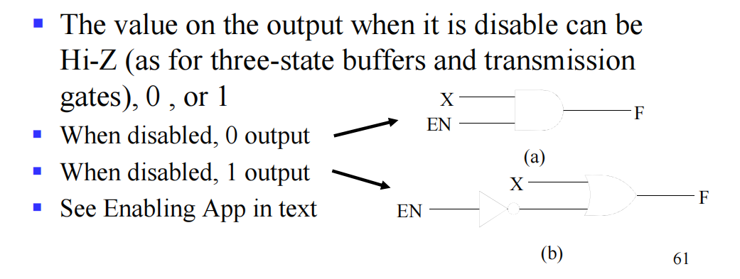
4. Enabling/Disabling: Using a control signal (\(EN\)) to either pass the input or block it.

Multiple-bit Rudimentary Functions (Buses)

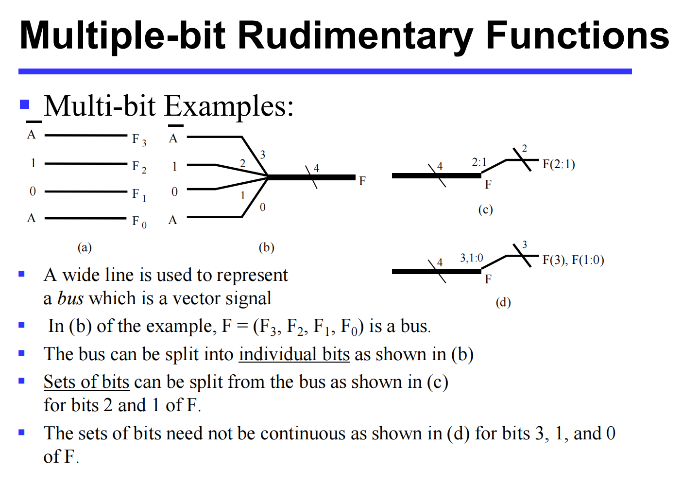
• 图片来自刘海风老师授课课件

3. Decoders

A decoder converts an \(n\)-bit input code into an \(m\)-bit output code (where \(m \le 2^n\)) such that each valid input code produces a unique active output.

General Characteristics

• Inputs/Outputs: \(n\)-to-\(m\) line decoders. Often \(m = 2^n\) to generate all possible minterms for the \(n\) input variables.

• Examples:

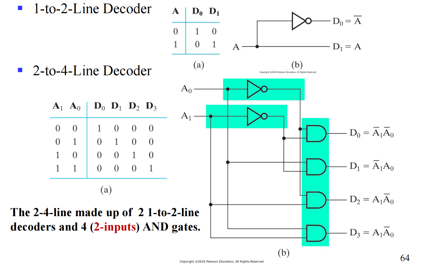
  • 1-to-2-Line Decoder: 1 input (\(A\)), 2 outputs (\(D_0 = \overline{A}\), \(D_1 = A\)). Requires 1 inverter.

  • 2-to-4-Line Decoder: Made up of two 1-to-2 decoders and four 2-input AND gates. Outputs map directly to minterms (e.g., \(D_0 = \overline{A}_1\overline{A}_0\)).

• 图片来自刘海风老师的授课课件

Decoder Expansion

Large decoders can be built hierarchically using smaller decoders.

• General Procedure for an \(n\)-to-\(2^n\) decoder:

  1. Split the \(n\) inputs into two groups (ideally equal, or differing by 1).

  2. Use two smaller decoders for these groups.

  3. Drive \(2^n\) output AND gates using the outputs of the smaller decoders.

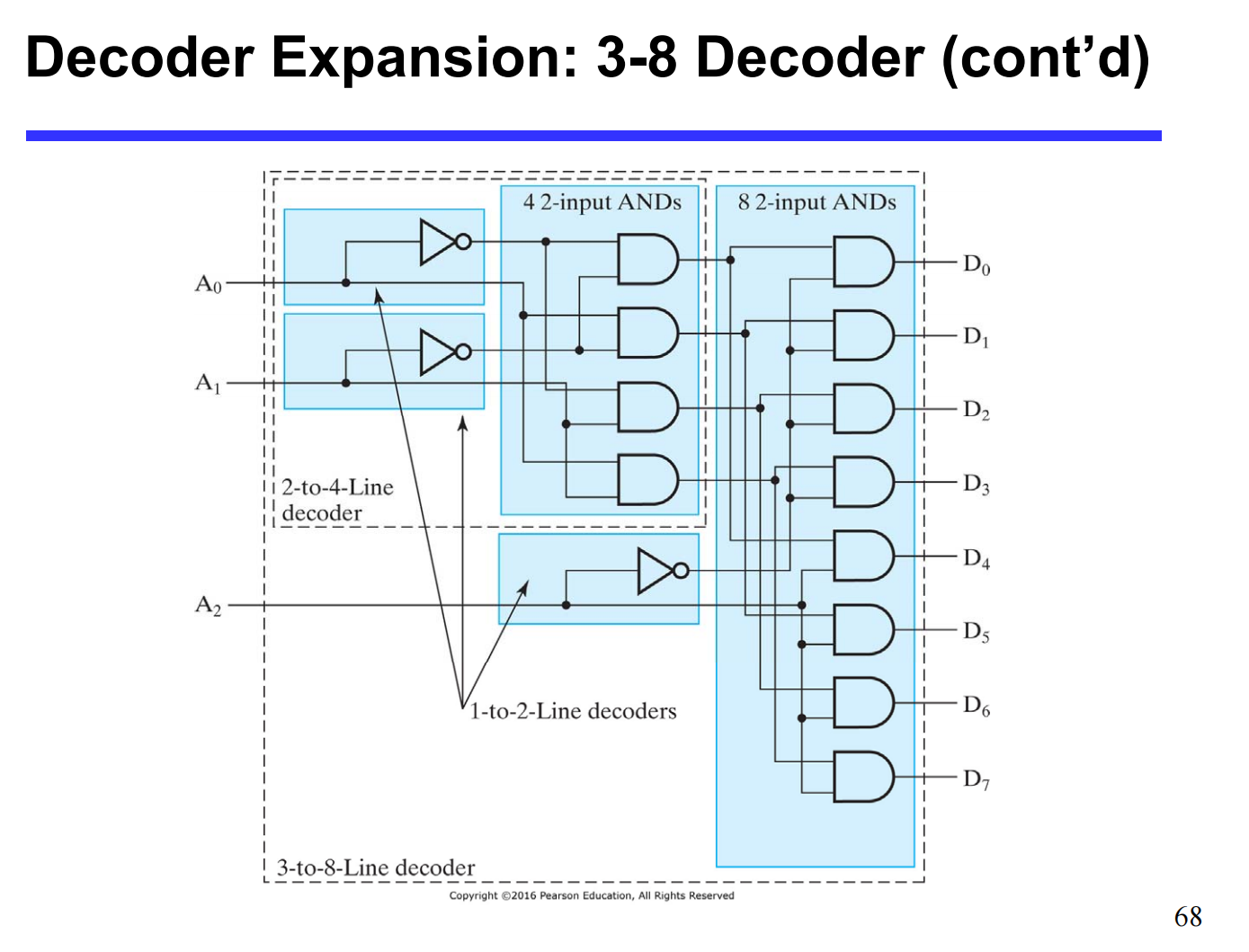
• Example (3-to-8 Decoder): Uses one 1-to-2 decoder (for \(A_2\)) and one 2-to-4 decoder (for \(A_1, A_0\)). Their outputs cross-connect into eight 2-input AND gates.

• 图片来自刘海风老师授课课件

Decoder with Enable (Demultiplexer)

• Attaching an enabling circuit to a decoder allows it to function as a Demultiplexer.

• Instead of just activating a designated output line based on an address, it routes the \(EN\) signal itself to that specific output line out of the \(2^n\) options.

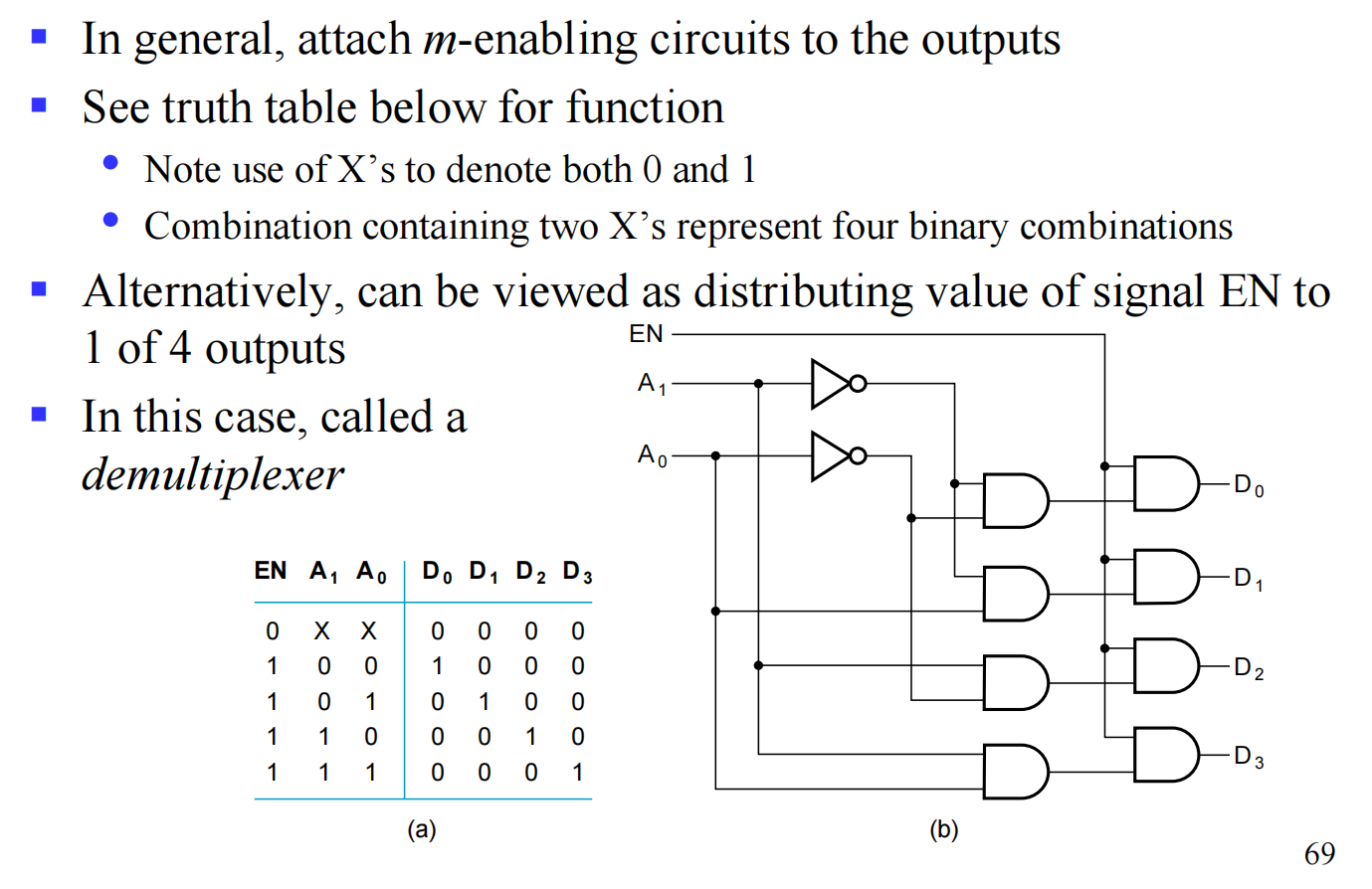
• 图片来自刘海风老师授课课件

Implementing Combinational Logic with Decoders

Since an \(n\)-to-\(2^n\) decoder generates all standard minterms, any boolean function can be implemented using:

• One \(n\)-to-\(2^n\) decoder to generate the minterms.

• \(m\) OR gates (one for each output function) to sum the required minterms.

BCD-to-Seven-Segment Decoder

A specific application that translates a 4-bit BCD input into 7 output signals to drive a 7-segment LED display.

• Common Anode (Active Low): LED anodes are tied to Vcc (logic 1). A segment turns ON when the decoder outputs a LOW (0).

• Common Cathode (Active High): LED cathodes are tied to Ground (logic 0). A segment turns ON when the decoder outputs a HIGH (1).

4. Encoders

The inverse of a decoder. It takes \(2^n\) (or fewer) inputs and compresses them into an \(n\)-bit output code.

Basic Encoder Issues

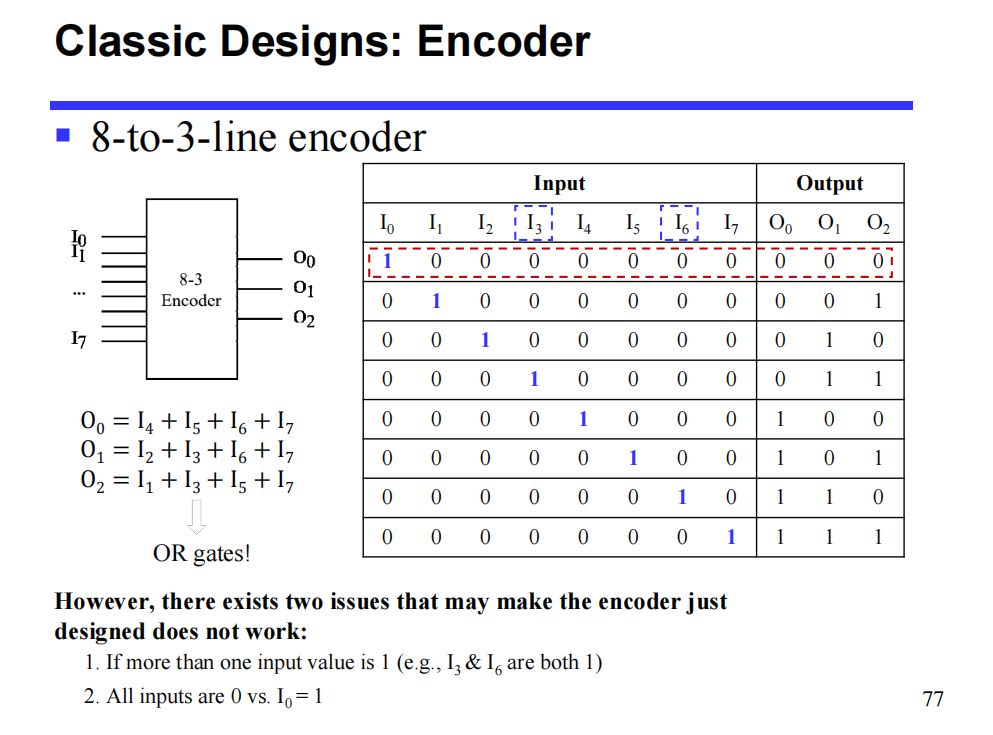
• 图片来自刘海风老师授课课件

Priority Encoder

Solves basic encoder issues by assigning priority to inputs.

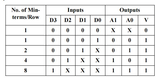
• 图片来自刘海风老师授课课件

• If multiple inputs are high, the output strictly corresponds to the input with the highest priority (e.g., \(D_3\) overrides \(D_2, D_1, D_0\)).

• Validity Bit (\(V\)): An additional output that goes high (1) if at least one input is active, distinguishing true 000 from an all-zero input state.

• Logic can be derived directly from a truth table utilizing "Don't Cares" (Xs) for lower-priority inputs.

5. Multiplexers (MUX)

A multiplexer is a digital switch that selects information from one of many input lines and directs it to a single output line.

MUX Structure

• Inputs/Outputs: \(n\) selection inputs (control lines), \(2^n\) information inputs (data lines), and 1 output.

• 2-to-1-Line MUX: Selects between \(I_0\) and \(I_1\) based on select line \(S\).

  • Equation: \(Y = \overline{S}I_0 + SI_1\)

  • Built using a 1-to-2 decoder, two enabling AND circuits, and an OR gate.

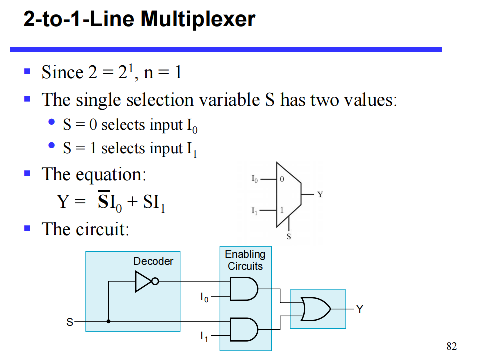
• 图片来自刘海风老师授课课件

• Expansion: A \(2^n\)-to-1 multiplexer combines an \(n\)-to-\(2^n\) decoder with a \(2^n \times 2\) AND-OR circuit.

  • Width Expansion: To select multi-bit vectors (buses) instead of single bits, use multiple MUXs in parallel sharing the same select lines (e.g., a Quad 4-to-1 MUX).

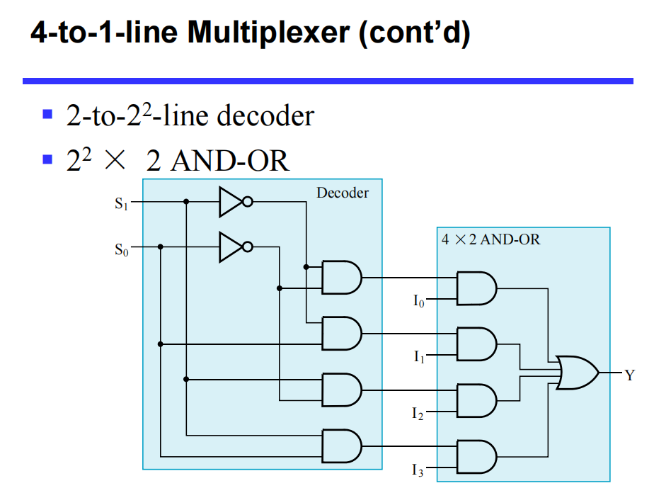
• 图片来自刘海风老师授课课件

Alternative MUX Implementations

Standard AND-OR logic can be gate-heavy. Alternative transistor-level designs reduce costs:

1. Three-State Logic: Replaces AND-OR gates with three-state buffers, resolving at a single output node. (Reduces gate input cost from 22 down to 18 for a 4-to-1 MUX).

   

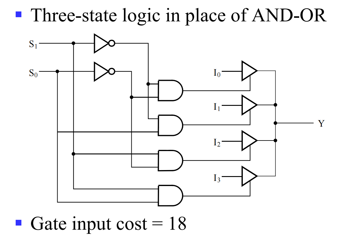
   • 图片来自刘海风老师授课课件

2. Distributed Decoding: Distributing decoding across three-state drivers further reduces cost (Cost = 14).

   

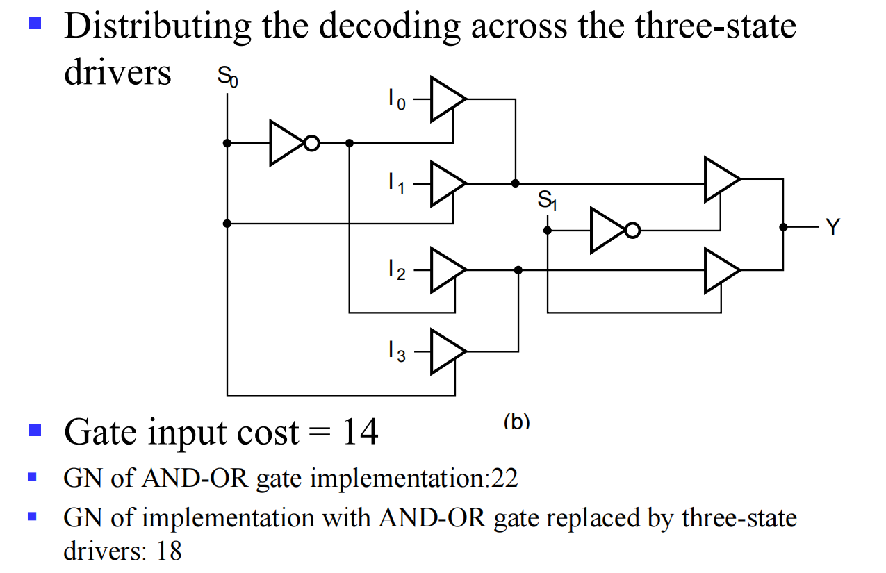
   • 图片来自刘海风老师授课课件

3. Transmission Gates (TG): Uses CMOS transmission gates for extremely efficient routing (Gate input cost = 8).

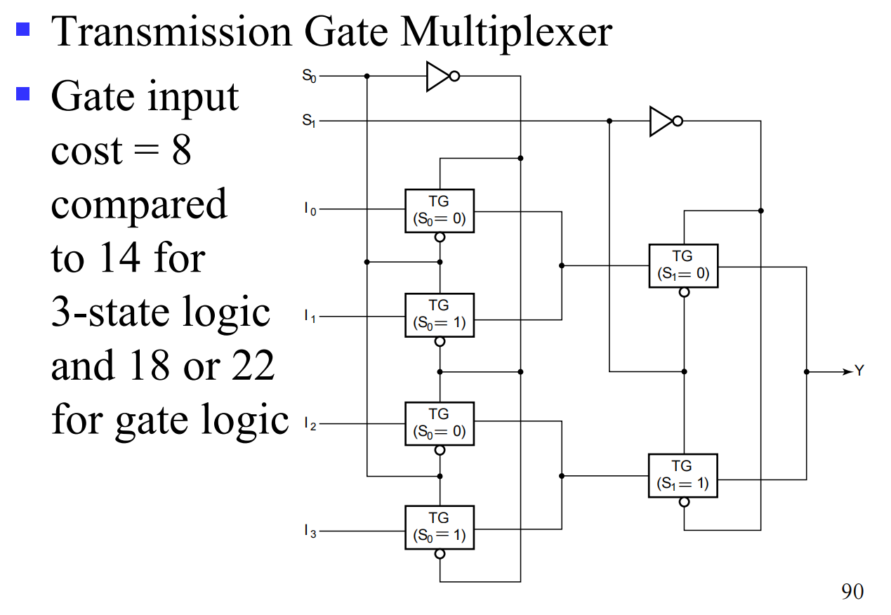
图片来自刘海风老师授课课件

Combinational Logic Implementation using Multiplexers

Multiplexers (MUXes) are not just data routing devices; they can be used as universal logic generators (essentially acting as hardware Look-Up Tables, or LUTs). Any boolean function can be implemented using a MUX without needing individual AND/OR gates.

There are two primary approaches to implementing combinational logic with MUXes, trading off between conceptual simplicity and hardware efficiency.

Approach 1: Direct Truth Table Mapping (Minterm Approach)

Concept: To implement \(m\) functions of \(n\) variables, we use an \(m\)-wide \(2^n\)-to-1-line multiplexer.

• Size mapping: The number of select lines exactly equals the number of input variables.

• Hardware cost: Requires a larger MUX.

Design Procedure:

1. Formulate the Truth Table: Derive the exact truth table for the desired output function(s).

2. Assign Selection Lines: Connect all \(n\) input variables directly to the multiplexer's selection inputs (\(S_{n-1}, \dots, S_0\)) in the exact order they appear in the truth table.

3. Value-Fix Data Inputs: Hardwire the data inputs (\(I_0, I_1, \dots, I_{2^n-1}\)) to constant logical values (0 or 1) corresponding directly to the output column of the truth table.

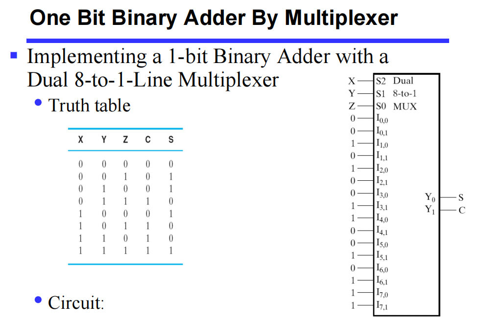
Example 1: 1-Bit Binary Adder (Approach 1)

• Specification: 3 input variables (\(X, Y, Z\)) and 2 output functions (\(S\) for Sum, \(C\) for Carry).

• Hardware Selection: Since \(n=3\) variables, we need a \(2^3 = 8\)-to-1 MUX. Since \(m=2\) outputs, we use a Dual 8-to-1-Line MUX.

• Implementation:

  • Select Lines: \(S_2 = X\), \(S_1 = Y\), \(S_0 = Z\).

  • By reading the truth table from top to bottom, we tie the data inputs directly to Vcc (1) or Ground (0):

    • Sum (\(Y_0\) or \(S\)): \(I_{0..7} = \{0, 1, 1, 0, 1, 0, 0, 1\}\)

    • Carry (\(Y_1\) or \(C\)): \(I_{0..7} = \{0, 0, 0, 1, 0, 1, 1, 1\}\)

---

Approach 2: Variable Folding (Optimized Approach)

Concept: You can implement any \(m\) functions of \(n+1\) variables using a MUX that is half the size: an \(m\)-wide \(2^n\)-to-1-line multiplexer plus a single inverter.

• Size mapping: The first \(n\) variables drive the selection lines. The final variable is evaluated at the data input lines.

• Hardware cost: Saves significant hardware area by utilizing a smaller MUX.

Design Procedure:

1. Formulate the Truth Table: Write out the standard truth table.

2. Separate into Pairs: Group the truth table rows into consecutive pairs based on the values of the first \(n\) variables.

3. Define Rudimentary Functions: For each pair, compare the desired output to the final input variable (let's call it \(V_{final}\)). The relationship will always reduce to one of four "rudimentary functions":

   • 0 (Output is always 0)

   • 1 (Output is always 1)

   • \(V_{final}\) (Output matches the final variable)

   • \(\overline{V_{final}}\) (Output is the inverse of the final variable)

4. Hardware Connection: * Connect the first \(n\) variables to the MUX select lines.

   • Connect the derived rudimentary functions to the MUX data inputs. Use the single inverter to generate \(\overline{V_{final}}\) if necessary.

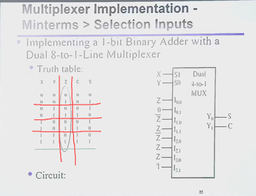
Example 2: 1-Bit Binary Adder (Approach 2)

• Specification: 3 input variables (\(X, Y, Z\)) and 2 output functions (\(S, C\)). Here, \(n+1 = 3\), meaning \(n=2\).

• Hardware Selection: We only need a \(2^2 = 4\)-to-1 MUX. For 2 outputs, we use a Dual 4-to-1-Line MUX.

• Derivation (Filling in the missing logic):

We use \(X\) and \(Y\) as select lines (\(S_1=X, S_0=Y\)). We evaluate the outputs \(S\) and \(C\) against the final variable \(Z\).

Select Lines (X,Y)	Final Var (Z)	Output S	Output C	Derivation for MUX Data Inputs (I0​…I3​)
0 0 (Pair 0)	0 1	0 1	0 0	For \(S\): Output matches \(Z \rightarrow\) \(I_0 = Z\) For \(C\): Output is always 0 \(\rightarrow\) \(I_0 = 0\)
0 1 (Pair 1)	0 1	1 0	0 1	For \(S\): Output is inverse of \(Z \rightarrow\) \(I_1 = \overline{Z}\) For \(C\): Output matches \(Z \rightarrow\) \(I_1 = Z\)
1 0 (Pair 2)	0 1	1 0	0 1	For \(S\): Output is inverse of \(Z \rightarrow\) \(I_2 = \overline{Z}\) For \(C\): Output matches \(Z \rightarrow\) \(I_2 = Z\)
1 1 (Pair 3)	0 1	0 1	1 1	For \(S\): Output matches \(Z \rightarrow\) \(I_3 = Z\) For \(C\): Output is always 1 \(\rightarrow\) \(I_3 = 1\)

• Implementation Result (Matches Image 4):

  • Select Lines: \(S_1 = X\), \(S_0 = Y\)

  • Data inputs for Sum (\(Y_0\)): \(I_0 = Z,\ I_1 = \overline{Z},\ I_2 = \overline{Z},\ I_3 = Z\)

  • Data inputs for Carry (\(Y_1\)): \(I_0 = 0,\ I_1 = Z,\ I_2 = Z,\ I_3 = 1\)

  • (Note: A single NOT gate is used to create the \(\overline{Z}\) signal fed into the \(S\) multiplexer).

---

Timing Analysis & Circuit Analysis

1. Circuit Delay Fundamentals

In reality, digital circuits do not respond instantaneously to input changes.

• Ideal Case: The output changes exactly at the same time as the input transitions.

• In Practice: There is a measurable time delay between an input changing and the output responding.

  • \(t_{pHL}\): The time it takes for the output to transition from High to Low after an input change.

  • \(t_{pLH}\): The time it takes for the output to transition from Low to High after an input change.

• Transmission Gate Delay: Delay is often measured from the point the input signal crosses the 50% voltage threshold to the point the output signal crosses the 50% threshold (rise-time delay).

2. Propagation and Contamination Delay

A combinational logic block has a window of time during which the outputs are unstable or transitioning. This is bounded by two key metrics:

• Propagation Delay (\(T_{pd}\)): The maximum delay from an input change to the final, stable output change. (The latest possible time the output will settle).

• Contamination Delay (\(T_{cd}\)): The minimum delay from an input change to any resulting output change. (The earliest possible time the output might start changing).

Reasons why \(T_{pd}\) and \(T_{cd}\) differ:

1. Transition asymmetries: Different rising (\(t_{pLH}\)) and falling (\(t_{pHL}\)) delays for a given gate.

2. Path variations: A circuit has multiple inputs and outputs, and signals may take different internal paths; some paths are physically faster than others.

3. Environmental factors: Operating temperature affects semiconductor performance (circuits generally slow down when hot and speed up when cold).

3. Path Analysis

To determine the overall timing characteristics of a complex circuit, we analyze the paths signals take through the logic gates.

• The Critical Path (Longest Path): Determines the overall Propagation Delay of the circuit. It is the path with the longest total delay.

  • \(T_{pd}\) of the circuit = \(\sum\) (all \(T_{pd}\) of circuit elements along the critical path)

• The Shortest Path: Determines the overall Contamination Delay of the circuit. It is the path with the shortest total delay.

  • \(T_{cd}\) of the circuit = \(\sum\) (all \(T_{cd}\) of circuit elements along the shortest path)

4. Race Hazards and Glitches

Differences in path delays can cause temporary errors in combinational logic.

• Race Hazard: Occurs when different signals taking different paths race to a single gate, arriving at slightly different times.

• Glitch: A temporary, unwanted change in the output state caused by a race hazard. It happens when a single input change causes multiple output changes.

Glitch Example: Consider the function \(F = A + \overline{A}\) implemented with an OR gate and an inverter.

• Ideally, \(A + \overline{A}\) is always \(1\).

• In reality: If \(A\) transitions from \(1\) to \(0\), the direct input to the OR gate becomes \(0\) immediately. However, the inverted input (\(\overline{A}\)) takes time to transition from \(0\) to \(1\) due to the inverter's delay.

• Result: For a brief moment, both inputs to the OR gate are \(0\), causing the output \(F\) to dip to \(0\) momentarily before recovering to \(1\). This is a glitch.

5. Analysis of Logic Circuits

The standard procedure for analyzing an existing logic circuit involves four steps:

1. Write the Boolean function for the circuit:

   • Begin with the input signals.

   • Define the relationships at the output of each gate.

   • Use algebraic optimization to simplify the final function.

2. Derive a truth table:

   • Define the exact relationships between all possible input combinations and the outputs.

3. Functional Analysis:

   • Define the plain-English function of each signal and the overall circuit (e.g., "F=1 if A!=B").

   • Draw the timing diagram of the circuit.

4. Verification:

   • Verify the correctness of the final design against the intended specifications.