03_Trees
1. Preliminaries & Terminology
A tree is a collection of nodes. The collection can be empty; otherwise, it consists of a distinguished node \(r\), called the root, and zero or more nonempty subtrees \(T_1, \dots, T_k\), each of whose roots are connected by a directed edge from \(r\).
Key Properties & Constraints:
-
Subtrees must not connect together. Therefore, every node in the tree is the root of some unique subtree.
-
A tree with \(N\) nodes always has exactly \(N-1\) edges (every node except the root has exactly one incoming edge).
Glossary of Terms:
-
Degree of a node: The number of subtrees (children) of a node.
-
Degree of a tree: The maximum degree among all nodes in the tree.
-
Parent & Children: A node that has subtrees is a parent; the roots of those subtrees are its children.
-
Siblings: Children sharing the same parent.
-
Leaf (Terminal Node): A node with a degree of 0 (no children).
-
Path: A unique sequence of nodes \(n_1, n_2, \dots, n_k\) such that \(n_i\) is the parent of \(n_{i+1}\).
-
Length of a path: The number of edges on the path (which is the number of nodes minus 1).
-
Depth of a node (\(n_i\)): The length of the unique path from the root to \(n_i\). The depth of the root is 0. (Counted top-down)
-
Height of a node (\(n_i\)): The length of the longest path from \(n_i\) to a leaf. The height of a leaf is 0. (Counted bottom-up)
-
Height (or Depth) of a tree: The height of the root, which equals the depth of the deepest leaf.
-
Ancestors / Descendants: Ancestors are all nodes along the path from the node up to the root. Descendants are all nodes in its subtrees.
Depth and Height can be the number of nodes or edges of the path, the actual concept should be confirmed in circumstances.
2. Tree Implementations
FirstChild-NextSibling Representation
Also known as the Left-Child Right-Sibling (LCRS) representation. Every node contains only two pointers, regardless of how many children it has:
-
FirstChild(Left pointer): Points to the node's first (leftmost) child. -
NextSibling(Right pointer): Points to the node's immediate right sibling.
Note: The representation of a general tree is not unique since the physical order of siblings can vary without changing the hierarchical structure.
3. Binary Trees
A binary tree is a tree in which no node can have more than two children.
3.1 Expression Trees (Syntax Trees)
Leaves are operands (e.g., \(A, B, c, d\)), and internal nodes are operators (e.g., \(+, *, /\)).
Prefix, Infix, and Postfix Conversions:
Traversing an expression tree yields different notations:
-
Pre-order Traversal \(\rightarrow\) Prefix Notation (Polish Notation): Operators precede operands (e.g., \(+ A * B C\)).
-
In-order Traversal \(\rightarrow\) Infix Notation: Standard human math (e.g., \(A + B * C\)). Note: Requires adding parentheses to preserve operator precedence.
-
Post-order Traversal \(\rightarrow\) Postfix Notation (Reverse Polish Notation): Operands precede operators (e.g., \(A B C * +\)). Ideal for computer evaluation.
Algorithmic Conversion (Without a Tree):
To manually or algorithmically convert between them, a Stack is used.
-
Infix to Postfix (Shunting Yard Algorithm)
-
Postfix to Tree Construction:
-
Read postfix expression left to right.
-
If operand, create a single-node tree and push to a stack.
-
If operator, pop two trees \(T_1\) (right child) and \(T_2\) (left child) from the stack. Create a new operator node, attach \(T_1\) and \(T_2\), and push the new tree back to the stack.
-
4. Tree Reconstruction: Deriving Structure from Traversals
A common and crucial problem in data structures is reconstructing the exact shape of a binary tree given its traversal sequences.
To uniquely identify a general binary tree, we must have the In-order traversal combined with either the Pre-order or Post-order traversal.
-
Pre-order / Post-order provides the Root of the current subtree.
-
In-order provides the Boundary (Partition), splitting the remaining nodes into Left and Right subtrees.
4.1 Reconstruction from Pre-order and In-order Traversals
The Core Logic:
-
Identify the Root: The first element in the Pre-order sequence is always the root of the current tree/subtree.
-
Partition the In-order Sequence: Find this root element in the In-order sequence. Everything to the left of this root in the In-order sequence belongs to the Left Subtree. Everything to the right belongs to the Right Subtree.
-
Count Subtree Sizes: Calculate the number of nodes in the Left Subtree (let's call this
L). -
Partition the Pre-order Sequence: In the Pre-order sequence, the next
Lelements immediately following the root belong to the Left Subtree. The elements after that belong to the Right Subtree. -
Recurse: Apply the same logic to the Left and Right subtrees.
Step-by-Step Example:
-
Pre-order:
[A, B, D, E, C, F] -
In-order:
[D, B, E, A, F, C] -
Step 1: Root is A (first in Pre-order).
-
Step 2: Find A in In-order:
[D, B, E] A [F, C].-
Left subtree In-order:
[D, B, E](Length \(L=3\)) -
Right subtree In-order:
[F, C]
-
-
Step 3: Use length \(L=3\) to split the remaining Pre-order elements
[B, D, E, C, F]:-
Left subtree Pre-order:
[B, D, E] -
Right subtree Pre-order:
[C, F]
-
-
Step 4: Recursively build the Left child using Pre:
[B,D,E]/ In:[D,B,E]and the Right child using Pre:[C,F]/ In:[F,C].
// Helper function to find the index of a value in an array
int findIndex(char arr[], int start, int end, char value) {
    for (int i = start; i <= end; i++) {
        if (arr[i] == value) return i;
    }
    return -1;
}

Tree buildTreePreIn(char pre[], int preStart, int preEnd,
                    char in[], int inStart, int inEnd) {
    // Base case: If the sequence is empty, return NULL
    if (preStart > preEnd || inStart > inEnd) return NULL;

    // 1. Create the root node from the first element of Pre-order
    Tree root = malloc(sizeof(struct TreeNode));
    root->Element = pre[preStart];

    // 2. Find the root's index in the In-order sequence
    int rootIndexInOrder = findIndex(in, inStart, inEnd, root->Element);

    // 3. Calculate the size of the left subtree
    int leftTreeSize = rootIndexInOrder - inStart;

    // 4. Recursively build left and right subtrees
    // Left child gets the immediate next 'leftTreeSize' elements in pre-order
    root->Left = buildTreePreIn(pre, preStart + 1, preStart + leftTreeSize,
                                in, inStart, rootIndexInOrder - 1);

    // Right child gets the rest of the elements in pre-order
    root->Right = buildTreePreIn(pre, preStart + leftTreeSize + 1, preEnd,
                                 in, rootIndexInOrder + 1, inEnd);

    return root;
}
4.2 Reconstruction from Post-order and In-order Traversals
The Core Logic:
The logic is almost identical to the Pre-order method, but we look at the end of the Post-order sequence to find the root.
-
Identify the Root: The last element in the Post-order sequence is the root.
-
Partition the In-order Sequence: Find this root in the In-order sequence to separate the Left and Right subtrees.
-
Count Subtree Sizes: Calculate the length of the Left Subtree (
L). -
Partition the Post-order Sequence: The first
Lelements of the Post-order sequence belong to the Left Subtree. The remaining elements (excluding the root at the very end) belong to the Right Subtree. -
Recurse: Apply the logic to both subtrees.
Tree buildTreePostIn(char post[], int postStart, int postEnd,
                     char in[], int inStart, int inEnd) {
    // Base case
    if (postStart > postEnd || inStart > inEnd) return NULL;

    // 1. Create the root node from the LAST element of Post-order
    Tree root = malloc(sizeof(struct TreeNode));
    root->Element = post[postEnd];

    // 2. Find the root in the In-order sequence
    int rootIndexInOrder = findIndex(in, inStart, inEnd, root->Element);

    // 3. Calculate the size of the left subtree
    int leftTreeSize = rootIndexInOrder - inStart;

    // 4. Recursively build left and right subtrees
    // Left child gets the first 'leftTreeSize' elements in post-order
    root->Left = buildTreePostIn(post, postStart, postStart + leftTreeSize - 1,
                                 in, inStart, rootIndexInOrder - 1);

    // Right child gets the elements after the left subtree up to the second-to-last element
    root->Right = buildTreePostIn(post, postStart + leftTreeSize, postEnd - 1,
                                  in, rootIndexInOrder + 1, inEnd);

    return root;
}
4.3 Why Pre-order + Post-order Fails
We cannot uniquely reconstruct a general binary tree using only Pre-order and Post-order sequences.
The Ambiguity of Single-Child Nodes:
The failure occurs when a parent node has exactly one child. Pre-order and Post-order traversals cannot distinguish whether that single child is a Left child or a Right child.
(Note: The only exception is a "Full Binary Tree" / "Strict Binary Tree" where every internal node has exactly two children. In this highly restricted case, Pre-order + Post-order can uniquely reconstruct the tree, as the single-child ambiguity does not exist.)
5. Tree Traversals (\(O(N)\) Time Complexity)
5.1 Recursive Implementations
// Pre-order: Visit Node -> Go Left -> Go Right
void preorder(tree_ptr tree) {
    if (tree) {
        visit(tree);
        preorder(tree->Left);
        preorder(tree->Right);
    }
}

// In-order: Go Left -> Visit Node -> Go Right
void inorder(tree_ptr tree) {
    if (tree) {
        inorder(tree->Left);
        visit(tree);
        inorder(tree->Right);
    }
}

// Post-order: Go Left -> Go Right -> Visit Node
void postorder(tree_ptr tree) {
    if (tree) {
        postorder(tree->Left);
        postorder(tree->Right);
        visit(tree);
    }
}
5.2 Iterative Implementations (Loop + Stack)
Recursive functions use the call stack. Iterative versions manually simulate this call stack.
1. Iterative Pre-order
void iter_preorder(tree_ptr tree) {
    if (!tree) return;
    Stack S = CreateStack(MAX_SIZE);
    Push(tree, S);

    while (!IsEmpty(S)) {
        tree_ptr curr = Pop(S);
        visit(curr);
        // Push Right first so Left is processed first (LIFO)
        if (curr->Right) Push(curr->Right, S);
        if (curr->Left) Push(curr->Left, S);
    }
}
2. Iterative In-order
void iter_inorder(tree_ptr tree) {
    Stack S = CreateStack(MAX_SIZE);
    tree_ptr curr = tree;

    while (curr != NULL || !IsEmpty(S)) {
        // Reach the left-most node of the current node
        while (curr != NULL) {
            Push(curr, S);
            curr = curr->Left;
        }
        // Current must be NULL at this point
        curr = Pop(S);
        visit(curr);        // Visit the node
        curr = curr->Right; // Now explore the right subtree
    }
}
3. Iterative Post-order (Using Two Stacks for clarity)
void iter_postorder(tree_ptr tree) {
    if (!tree) return;
    Stack S1 = CreateStack(MAX_SIZE); // Traversal stack
    Stack S2 = CreateStack(MAX_SIZE); // Output stack
    Push(tree, S1);

    while (!IsEmpty(S1)) {
        tree_ptr curr = Pop(S1);
        Push(curr, S2);

        // Push left then right (so right is popped and processed first into S2)
        if (curr->Left) Push(curr->Left, S1);
        if (curr->Right) Push(curr->Right, S1);
    }

    // S2 now contains the post-order sequence
    while (!IsEmpty(S2)) {
        visit(Pop(S2));
    }
}
5.3 Level-order Traversal (Breadth-First)
Uses a Queue instead of a Stack.
void levelorder(tree_ptr tree) {
    if (!tree) return;
    Queue Q = CreateQueue(MAX_SIZE);
    Enqueue(tree, Q);

    while (!IsEmpty(Q)) {
        tree_ptr curr = Dequeue(Q);
        visit(curr);
        if (curr->Left) Enqueue(curr->Left, Q);
        if (curr->Right) Enqueue(curr->Right, Q);
    }
}
6. Practical Applications of Traversals
1. Directory Listing (Pre-order Application)
When listing a hierarchical file system, we print the parent directory first, then recursively print its contents.
-
Logic: Visit node -> recursively visit children.
-
Depth Tracking: A variable
Depthis passed down the recursion to determine how many 'tabs' to indent, visually representing the hierarchy. To abstract this from the user, a public wrapper functionListDirectory(DirOrFile D)is used, which privately callsListDir(D, 0)starting at depth 0.
2. Calculating Directory Size (Post-order Application)
To know the size of a folder, we must first calculate the size of all files and folders inside it, sum them up, and then return the total to the parent.
-
Logic: Recursively process children -> accumulate values -> resolve parent node.
-
Complexity: \(T(N) = O(N)\) because every file and directory is visited exactly once.
7. Threaded Binary Trees
7.1 The Problem: Wasted Space and Traversal Overhead
In a standard binary tree with \(N\) nodes, there are \(2N\) total link fields (left and right pointers). However, only \(N-1\) of these are actually used to connect nodes (the edges). This leaves exactly \(N+1\) NULL pointers wasting memory space.
Furthermore, performing an iterative in-order traversal traditionally requires an external Stack (or parent pointers) to trace back to parent nodes, which consumes additional dynamic memory and overhead.
7.2 The Solution: "Threading" the Tree
Threaded Binary Trees solve this by repurposing those \(N+1\) unused NULL pointers to point to the node's in-order predecessor and in-order successor. These repurposed pointers are called threads.
The Three Rules of Threading:
-
Rule 1 (Left Threads): If a node's
Leftpointer isNULL, replace it with a pointer (thread) to its in-order predecessor. -
Rule 2 (Right Threads): If a node's
Rightpointer isNULL, replace it with a pointer (thread) to its in-order successor. -
Rule 3 (The Head Node): There must not be any "loose" threads (dangling pointers). A threaded binary tree must have a dummy head node to manage the extreme ends of the tree:
-
The head node's
Leftchild points to the actual root of the tree. -
The head node's
Rightchild points to itself. -
The left thread of the very first node in the in-order sequence points to the head node.
-
The right thread of the very last node in the in-order sequence points to the head node.
-
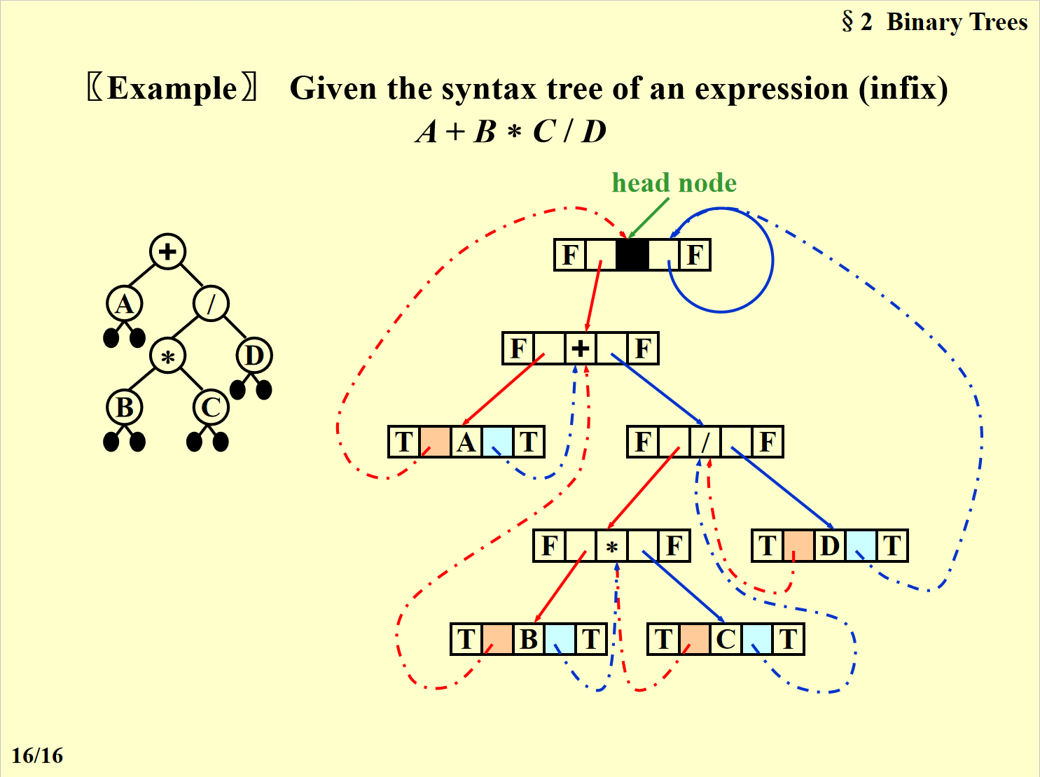
- diagram from the courseware of Mr. He qinming (何钦铭)
7.3 Data Structure Implementation
To differentiate between a normal child pointer and a "thread", we must add two boolean flags to each node.
// Defines the structure for a Threaded Tree Node
typedef struct ThreadedTreeNode *PtrToThreadedNode;
typedef struct PtrToThreadedNode ThreadedTree;

typedef struct ThreadedTreeNode {
    int LeftThread;       /* 1 (TRUE) if Left is a thread, 0 (FALSE) if it's a child */
    ThreadedTree Left;    /* Pointer to left child OR predecessor */

    ElementType Element;  /* The data payload */

    int RightThread;      /* 1 (TRUE) if Right is a thread, 0 (FALSE) if it's a child */
    ThreadedTree Right;   /* Pointer to right child OR successor */
} ThreadedTreeNode;
7.4 How to Traverse a Threaded Tree
The primary advantage of a threaded tree is that we can perform an in-order traversal without recursion and without a stack, resulting in \(O(1)\) extra space complexity.
Logic to find the In-order Successor of any node X:
-
If
X->RightThread == TRUE: The successor is simplyX->Right. -
If
X->RightThread == FALSE:Xhas a right subtree. The in-order successor is the left-most node in that right subtree.
Iterative In-order Traversal Code (Using Threads):
// Find the left-most node starting from a given node
ThreadedTree FirstNode(ThreadedTree node) {
    while (node->LeftThread == 0) { // While it has a real left child
        node = node->Left;
    }
    return node;
}

// Find the next node in in-order sequence
ThreadedTree NextNode(ThreadedTree node) {
    if (node->RightThread == 1) {   // If right pointer is a thread
        return node->Right;         // Just follow the thread
    } else {                        // If right pointer is a real child
        return FirstNode(node->Right); // Go right, then all the way left
    }
}

// Full In-order Traversal without Stack
void InorderTraversal_Threaded(ThreadedTree HeadNode) {
    ThreadedTree curr = FirstNode(HeadNode->Left); // Start at the true first node

    while (curr != HeadNode) { // Loop until we thread back to the dummy head
        visit(curr);
        curr = NextNode(curr);
    }
}
8. Binary Trees: Fundamentals
8.1 Core Concept
Unlike a general tree where the order of children may not matter, a binary tree is strictly positional. In a binary tree, the left child and the right child are distinct. Even if a node has only one child, it must be explicitly designated as either a left child or a right child.
-
Skewed Binary Tree: A tree where every node has only one child (either all left children or all right children). It degenerates into a linear linked list.
-
Complete Binary Tree: A binary tree where all levels except possibly the last are fully filled, and all leaf nodes on the last level are justified to the left.
8.2 Mathematical Properties of Binary Trees
Understanding the structural limits of binary trees is crucial for analyzing algorithm efficiency.
-
Maximum Nodes on a Level: The maximum number of nodes on level \(i\) is \(2^{i-1}\) (where \(i \ge 1\), root is level 1).
-
Maximum Total Nodes: The maximum number of nodes in a binary tree of depth \(k\) is \(2^k - 1\) (where \(k \ge 1\)).
-
Node Degree Relationship (\(n_0 = n_2 + 1\)): For any nonempty binary tree, the number of leaf nodes (nodes with 0 children, denoted as \(n_0\)) is always exactly one more than the number of nodes with 2 children (denoted as \(n_2\)).
Proof of \(n_0 = n_2 + 1\):
Let \(n\) be the total number of nodes, and \(n_1\) be the number of nodes of degree 1.
Therefore, the total number of nodes is: \(n = n_0 + n_1 + n_2\)
Let \(B\) be the total number of branches (edges). Every node except the root has exactly one incoming branch.
Therefore: \(n = B + 1\)
Branches only originate from nodes of degree 1 (1 branch each) and nodes of degree 2 (2 branches each).
Therefore: \(B = n_1 + 2n_2\)
Substituting equation (3) into equation (2) gives: \(n = n_1 + 2n_2 + 1\)
Setting this equal to equation (1): \(n_0 + n_1 + n_2 = n_1 + 2n_2 + 1\)
Simplifying yields: \(n_0 = n_2 + 1\)