10 · Magnetic Dipoles and Magnetic Materials
Course index · Previous · Next
1. Magnetic moment: origin and response
A current loop, an atom, or a permanent magnet can have a magnetic dipole moment. For a planar coil,
The moment has units A·m² = J/T. Parallel alignment minimizes energy; zero torque at anti-alignment is unstable. For a fixed small moment in a nonuniform field, \(\mathbf F=\nabla(\boldsymbol\mu\cdot\mathbf B)\): translational attraction or repulsion requires a field gradient.
Atomic magnetism involves orbital angular momentum(轨道角动量) and spin(自旋). For a classical charge orbit, \(\boldsymbol\mu_{\mathrm{orb}}=(q/2m)\mathbf L\). Electron spin has its own gyromagnetic factor; it is intrinsic angular momentum, not a literal charged sphere spinning about an axis. Microscopic magnetic moments do not in general arise only from orbital currents.
2. Circular arc, coil, and dipole field
At the center of an arc of radius \(R\) subtending angle \(\varphi\) in radians,
The field is normal to the arc's plane. A full loop gives \(\mu_0i/(2R)\); radial connecting segments contribute zero at the center because \(d\boldsymbol\ell\parallel\mathbf R\).
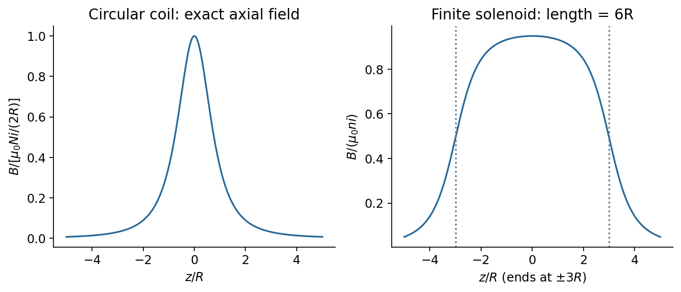
For an \(N\)-turn circular coil, symmetry cancels transverse components on its axis. Biot–Savart gives
Its limits are \(B_z(0)=\mu_0Ni/(2R)\) and \(B_z\simeq\mu_0\mu/(2\pi z^3)\) for \(z\gg R\), with \(\mu=Ni\pi R^2\). Matching limiting cases can suggest this expression, but does not prove the interpolation; the integral supplies the proof.
For a localized magnetic dipole at far-field distance \(r\),
It has the same far-field angular structure as an electric dipole, while magnetic flux still has zero divergence. This expression is not the finite coil's near field.
Finite-solenoid check
Class 10 adds the fields of circular turns to recover the solenoid result. For radius \(R\), length \(\ell\), and center \(z=0\),
For \(\ell\gg R\), the field deep inside tends to \(\mu_0ni\) and near an end to \(\mu_0ni/2\). This explains the limits of the infinite-solenoid approximation.
3. Magnetization(磁化强度)
Define net magnetic moment per unit volume:
Magnetization describes both response to a field and a source of additional magnetic field. A useful macroscopic convention is
For a linear isotropic material, \(\mathbf M=\chi_m\mathbf H\) and \(\mu_r=1+\chi_m\). This linear relation does not describe an entire ferromagnetic hysteresis loop; sample shape and demagnetizing fields can make the internal \(\mathbf H\) differ from the applied field.
4. Paramagnetism(顺磁性) and Curie's law
Independent permanent moments are disordered at zero applied field by thermal fluctuations. A field biases them toward lower-energy orientations.
The slides' two-state model allows moments parallel or antiparallel to a field of magnitude \(B\):
For number density \(n\),
At \(x\ll1\), \(\tanh x\simeq x\), giving \(M\simeq n\mu^2B/(k_BT)\propto B/T\) (Curie's law). At large positive \(x\), \(M\to n\mu\): saturation prevents indefinite linear growth.
The coefficient depends on the microscopic allowed orientations. A classical freely rotating dipole has a different weak-field coefficient from this two-state model; the slides' proportionality should not be treated as a universal numerical constant. Weak paramagnets are attracted toward stronger fields because the aligned moments lower their energy there.
5. Diamagnetism(抗磁性)
An applied field induces a moment opposing the field; weak diamagnets have \(\chi_m<0\) and tend to move toward weaker fields. Diamagnetic contributions exist even when stronger magnetic responses mask them.
In the slide's classical fixed-radius orbital model, slowly switching on an axial field induces an azimuthal electric field. Its torque changes the orbit, leading to
Both initially clockwise and counterclockwise orbits acquire the same opposing correction. This is a qualitative induced-current model, not a complete classical explanation of atomic magnetism. The changing field's electric component changes the speed; a static magnetic Lorentz force alone does not do that work.
Superconducting screening is a much stronger, distinct quantum response; magnetic levitation does not imply that ordinary weak diamagnetism and superconductivity have the same microscopic origin.
6. Collective magnetism, domains, and hysteresis
A schematic interaction model uses unit spin directions \(\mathbf s_j\) and moment magnitude \(\mu\):
For \(J>0\), aligned neighboring spins lower the interaction energy. Exchange interactions, rather than only the classical dipole field, are central to ordinary ferromagnetism. Thermal agitation competes with ordering; equilibrium minimizes the free energy \(F=U-TS\), not energy alone.
- Below a Curie temperature \(T_C\), a ferromagnet can have spontaneous magnetization in zero applied field.
- Above \(T_C\), long-range ferromagnetic order disappears. The transition temperature is related to an interaction-energy scale, with details depending on structure and dimensionality.
- A macroscopic specimen can contain domains(磁畴) with different magnetization directions, giving little net moment even while each domain is ordered.
- Applied fields move domain walls and rotate domains. Irreversibility produces hysteresis(磁滞), including remanence and a coercive field needed to reverse magnetization.
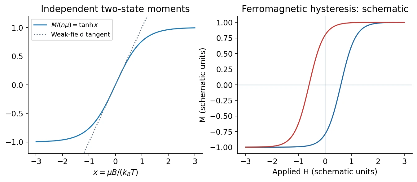
The hysteresis curves are illustrative, not measured data or a microscopic model.
中文提示:顺磁体的各磁矩主要响应外场;铁磁体还依赖磁矩之间的集体相互作用。铁磁体“总磁矩为零”可能只是磁畴抵消,并不等于局部无序。
Broader classification and classroom context
| Response / order | Distinguishing feature |
|---|---|
| Diamagnetic | Induced opposing moment; weak negative susceptibility. |
| Paramagnetic | Field-biased moments without spontaneous long-range order in the considered regime. |
| Ferromagnetic | Parallel collective order and possible spontaneous net magnetization. |
| Antiferromagnetic(反铁磁) | Opposing ordered sublattices with compensated moments in the simple case. |
| Ferrimagnetic(亚铁磁) | Opposing sublattices with unequal moments, leaving a net moment. |
The spin-glass introduction concerns disorder and competing interactions that frustrate simple ordering, rather than just random high-temperature spins. The Nobel 2021 background explains that context; detailed spin-glass theory is not part of these lessons.
Class 11 completes the phase-transition discussion: an ordered state selects a magnetization direction and breaks a symmetry of the disordered phase. It then introduces the anomalous Hall effect: magnetization can add a transverse response beyond the ordinary applied-field term. A remanently magnetized suitable material can retain that response at zero applied field. The quantum anomalous Hall effect is a distinct quantized regime in appropriate magnetic topological systems, not a property of every ferromagnet. The classroom's example is Chang et al., Science 340, 167–170 (2013); no band-topology calculation is required here.
Related homework(知识点应用)
- Ch. 9, Ex. 2 · Ring superposition for a spherical shell.
- Ch. 10, Ex. 1 · Far-field dipole derivation and interaction energy.
Sources and checks
Lecture 10 pp. 5–15: moments and coil fields; pp. 16–27: material response; p. 29 and the opening approximately 22 minutes of class 11: anomalous Hall and ordering. The finite-solenoid integration and microscopic angular-momentum discussion come from class 10. Check field uniformity, far-field limits, the chosen moment model, and whether a response is induced or spontaneous.