14 · Maxwell's Equations and Electromagnetic Waves

1. Why magnetostatic Ampère's law is incomplete

For any smooth vector field, \(\nabla\cdot(\nabla\times\mathbf B)=0\). Taking the divergence of \(\nabla\times\mathbf B=\mu_0\mathbf J\) would therefore require \(\nabla\cdot\mathbf J=0\). But charge conservation gives

\[ \nabla\cdot\mathbf J=-\frac{\partial\rho_q}{\partial t}, \]

which need not vanish during charging. Gauss's law identifies a correction:

\[ \frac{\partial\rho_q}{\partial t}=\epsilon_0\nabla\cdot\frac{\partial\mathbf E}{\partial t}. \]

The Ampère–Maxwell law is

\[ \boxed{\nabla\times\mathbf B =\mu_0\mathbf J+\mu_0\epsilon_0\frac{\partial\mathbf E}{\partial t},\qquad \mathbf J_d=\epsilon_0\frac{\partial\mathbf E}{\partial t}.} \]

The new term is the vacuum displacement-current density（位移电流密度）. Its divergence restores compatibility with charge conservation. That consistency argument motivates the term; it is not, by itself, a uniqueness proof excluding every imaginable additional divergence-free field term.

2. Charging capacitor: independence of spanning surface

For a fixed boundary curve \(C\), the integral law is

\[ \boxed{\oint_C\mathbf B\cdot d\boldsymbol\ell =\mu_0\int_S\mathbf J\cdot d\mathbf A +\mu_0\epsilon_0\frac d{dt}\int_S\mathbf E\cdot d\mathbf A.} \]

Choose one spanning surface that cuts a charging wire and another that bows between the capacitor plates. The first receives conduction current \(i\); the second receives no conduction through the vacuum gap. Yet both must predict the same circulation.

Neglecting edge effects, \(E=Q/(\epsilon_0A)\) in the gap, so

\[ I_d=\epsilon_0\frac{d(EA)}{dt}=\frac{dQ}{dt}=i. \]

The two surfaces agree once displacement current is included. It is not literal charge transport across the vacuum gap. Statements that exterior \(E\) is zero are only the ideal capacitor approximation; the full law counts both terms wherever they occur.

3. Maxwell's four equations in vacuum

Here \(\rho_q\) and \(\mathbf J\) are total physical charge and current densities. Integral forms use fixed surfaces/contours, outward normals on closed surfaces, and the right-hand orientation on open ones.

Law	Differential form	Integral form
Electric Gauss	\(\nabla\cdot\mathbf E=\rho_q/\epsilon_0\)	\(\oint_S\mathbf E\cdot d\mathbf A=Q_{\mathrm{enc}}/\epsilon_0\)
Magnetic Gauss	\(\nabla\cdot\mathbf B=0\)	\(\oint_S\mathbf B\cdot d\mathbf A=0\)
Faraday	\(\nabla\times\mathbf E=-\partial_t\mathbf B\)	\(\oint_C\mathbf E\cdot d\boldsymbol\ell=-d\Phi_B/dt\)
Ampère–Maxwell	\(\nabla\times\mathbf B=\mu_0\mathbf J+\mu_0\epsilon_0\partial_t\mathbf E\)	\(\oint_C\mathbf B\cdot d\boldsymbol\ell=\mu_0I_{\mathrm{enc}}+\mu_0\epsilon_0d\Phi_E/dt\)

Together with the Lorentz force \(\mathbf F=q(\mathbf E+\mathbf v\times\mathbf B)\), these describe classical electromagnetic interactions once sources, initial data, and boundary conditions are supplied. In materials, constitutive response is also needed; \(\mathbf D\) and \(\mathbf H\) allow a macroscopic formulation in terms of free sources.

The electric and magnetic equations are not fully source-symmetric: electric charges are sources of electric divergence, while classical Maxwell theory contains no magnetic charge. The course mentions magnetic monopoles as a theoretical possibility, not an observed source inserted into these equations.

4. Deriving the source-free wave equation

In vacuum with \(\rho_q=0\) and \(\mathbf J=0\),

\[ \nabla\cdot\mathbf E=\nabla\cdot\mathbf B=0,\qquad \nabla\times\mathbf E=-\partial_t\mathbf B,\qquad \nabla\times\mathbf B=\mu_0\epsilon_0\partial_t\mathbf E. \]

Take the curl of Faraday's law and use the vector identity

\[ \nabla\times(\nabla\times\mathbf E) =\nabla(\nabla\cdot\mathbf E)-\nabla^2\mathbf E. \]

This yields, and the magnetic calculation similarly yields,

\[ \boxed{\nabla^2\mathbf E=\frac1{c^2}\partial_t^2\mathbf E,\qquad \nabla^2\mathbf B=\frac1{c^2}\partial_t^2\mathbf B,\qquad c=\frac1{\sqrt{\mu_0\epsilon_0}}.} \]

Each Cartesian field component satisfies a wave equation. The oscillating quantities are field values, not a material medium. Eliminating the coupling to obtain wave equations does not eliminate the original Maxwell constraints on allowable solutions.

5. Plane waves: dispersion and transverse structure

Write

\[ \mathbf E=\mathbf E_m\cos(\mathbf k\cdot\mathbf r-\omega t+\alpha),\qquad \mathbf B=\mathbf B_m\cos(\mathbf k\cdot\mathbf r-\omega t+\alpha). \]

The wave equation gives \(\omega=ck\), with \(k=2\pi/\lambda\) and \(\omega=2\pi f\). The remaining Maxwell equations impose

\[ \boxed{\mathbf k\cdot\mathbf E_m=\mathbf k\cdot\mathbf B_m=0,\qquad \mathbf B=\frac1c\hat{\mathbf k}\times\mathbf E.} \]

For a single traveling vacuum plane wave, \(\mathbf E\), \(\mathbf B\), and propagation are mutually perpendicular; \(E=cB\), and the two fields are in phase. For propagation along \(+x\), a choice is \(\mathbf E\parallel+\hat{\mathbf y}\) and \(\mathbf B\parallel+\hat{\mathbf z}\). Reversing either transverse field reverses the direction of energy flow.

A drawing of sinusoidal field arrows represents values at points on the propagation axis, not the sideways path of a particle. The simple \(E=cB\) relation need not hold for arbitrary superpositions, standing waves, or near fields.

6. Energy flux, intensity, and spreading

The Poynting vector（坡印廷矢量） in vacuum is

\[ \boxed{\mathbf S=\frac1{\mu_0}\mathbf E\times\mathbf B,\qquad [S]=\mathrm{W/m^2}.} \]

For fields in vacuum or the nonmagnetic Ohmic model used in the homework, local energy conservation is Poynting's theorem:

\[ \boxed{\frac{\partial u}{\partial t}+\nabla\cdot\mathbf S=-\mathbf J\cdot\mathbf E, \qquad u=\frac{\epsilon_0E^2}{2}+\frac{B^2}{2\mu_0}.} \]

It follows by dotting the Ampère–Maxwell equation with \(\mathbf E/\mu_0\), Faraday's equation with \(\mathbf B/\mu_0\), and using \(\nabla\cdot(\mathbf E\times\mathbf B)=\mathbf B\cdot(\nabla\times\mathbf E)-\mathbf E\cdot(\nabla\times\mathbf B)\). The term \(\mathbf J\cdot\mathbf E\) is field power delivered to matter; for \(\mathbf J=\sigma\mathbf E\) it is positive Joule heating. 场能变化、流出边界的能流和物质获得的功率必须一起记账。 Ch. 14, Ex. 3 applies this law to inward energy flow into a resistive wire.

For a traveling plane wave,

\[ u_E=\frac12\epsilon_0E^2=\frac{B^2}{2\mu_0}=u_B,\qquad S=c(u_E+u_B)=\epsilon_0cE^2. \]

The time-averaged intensity of a sinusoid is

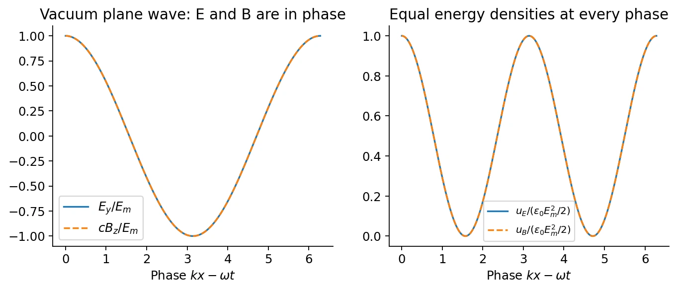
\[ \boxed{I=\langle S\rangle =\frac12\epsilon_0cE_m^2 =\frac{cB_m^2}{2\mu_0}.} \]

In-phase electric and magnetic fields of a vacuum plane wave, with equal instantaneous electric and magnetic energy densities

中文提示：行进平面波的电场能和磁场能同时达到峰值，且始终相等；LC 电路中两种能量则交替转换。不要把这两幅图混为一谈。

For an isotropic point source radiating power \(P\) into lossless space,

\[ I(r)=\frac{P}{4\pi r^2}. \]

Far-field wave amplitudes consequently scale as \(1/r\). A dipole antenna is not isotropic: radiation depends on direction, although far-field radial spreading still gives \(1/r^2\) intensity along a fixed direction. Near-field terms have different distance dependence.

7. Generation and the electromagnetic spectrum

An LC oscillator coupled through a transmission line to a dipole antenna drives oscillating charge/current. Accelerating charges radiate at the drive frequency; receiver circuitry responds to the arriving fields. A source is needed to maintain radiation and compensate losses.

Radio, microwave, infrared, visible, ultraviolet, X-ray, and gamma radiation belong to the same electromagnetic spectrum, differing principally in frequency and wavelength. In vacuum they share speed \(c\); differences in propagation through matter require the material's frequency-dependent response. Momentum transport and radiation pressure are developed at the beginning of class 15.

Sources and checks

Lecture 14 pp. 3–13: Maxwell correction and equations; pp. 14–24: wave equation and plane-wave constraints; pp. 25–29: generation and energy transport; p. 33: Poynting vector. Radiation-pressure appendix pp. 34–37 is treated with the class-15 discussion. Check surface independence, vacuum/source-free assumptions, \(E\) versus \(E_m\), and amplitude versus intensity decay.