12 · Inductance, RL Circuits, and Magnetic Energy

Course index · Previous · Next

1. Flux linkage and self-inductance（自感）

A current creates magnetic flux through its own circuit. For fixed geometry and linear magnetic response,

\[ \boxed{\Lambda=Li,\qquad L=\frac\Lambda i,\qquad 1\ \mathrm H=1\ \mathrm{Wb/A}=1\ \mathrm{V\,s/A}.} \]

For \(N\) turns all linking the same flux, \(\Lambda=N\Phi_B\). The total flux linkage, not one turn's flux, defines the inductance. The slides initially assume vacuum/air cores without nearby magnetic materials; in general \(L\) depends on material response as well as geometry and can become nonlinear.

Long solenoid

With \(n=N/\ell\), cross-sectional area \(A\), and negligible end fields,

\[ B=\mu_0ni,\qquad \Lambda=NAB=\mu_0n^2\ell A\,i, \]

so

\[ \boxed{L=\mu_0n^2\ell A=\frac{\mu_0N^2A}{\ell},\qquad \frac L\ell=\mu_0n^2A.} \]

The square in \(N\) reflects both a stronger source field and more turns linking that field. The expression assumes a tightly wound solenoid with length much larger than radius.

2. Self-induced emf and terminal voltage

Faraday's law gives

\[ \mathcal E_L=-\frac{d\Lambda}{dt}=-L\frac{di}{dt} \]

for constant \(L\). The self-emf opposes the change in current: it opposes an increase but supports the existing current during a decrease.

With current entering the labeled positive terminal, the ideal inductor's passive terminal voltage is

\[ \boxed{v_L=L\frac{di}{dt}.} \]

The opposing emf and the terminal voltage use different sign conventions; they are not competing laws. A winding with resistance \(r\) has \(v=ri+L\,di/dt\). In a nonlinear core one must use \(d\Lambda/dt\), not assume a constant \(L\).

The winding's interior field can be nonconservative. Terminal voltage is a lumped-circuit quantity defined with a consistent lead path outside the strongly changing-flux region; it is not proof that a global electrostatic potential exists throughout the coil.

3. RL switch-on and decay

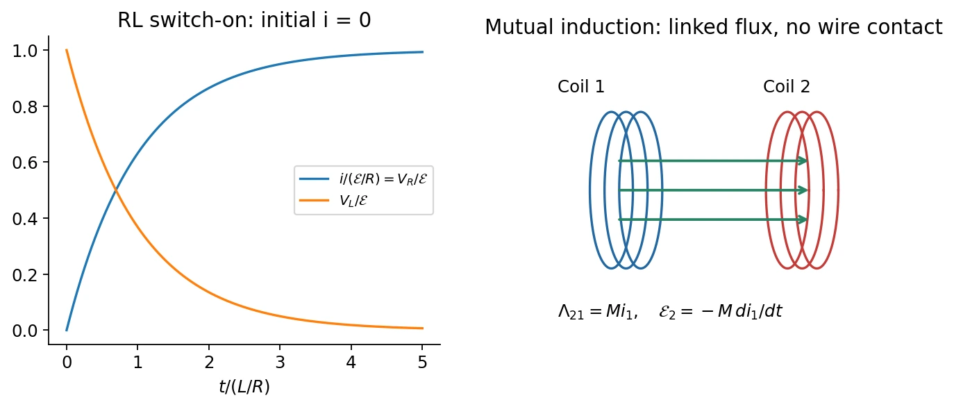
For an initially current-free series circuit,

\[ L\frac{di}{dt}+Ri=\mathcal E,\qquad \tau_L=\frac LR. \]

The general constant-source solution is

\[ i(t)=\frac{\mathcal E}{R}+ \left(i(0)-\frac{\mathcal E}{R}\right)e^{-t/\tau_L}. \]

For \(i(0)=0\),

\[ \boxed{i=\frac{\mathcal E}{R}(1-e^{-t/\tau_L}),\qquad v_R=\mathcal E(1-e^{-t/\tau_L}),\qquad v_L=\mathcal E e^{-t/\tau_L}.} \]

At \(t=0^+\) the inductor supports the applied voltage and current is still zero. At long times an ideal inductor has zero voltage drop and acts as a DC short circuit. Current cannot jump without an impulsive voltage.

If the source is removed while a closed resistive discharge path remains,

\[ i(t)=i_0e^{-t/\tau_L},\qquad v_L=-Ri. \]

Opening an inductive circuit without a suitable path can instead generate a large voltage; an ideal exponential-decay formula presupposes the specified discharge circuit.

Feature	RC circuit	RL circuit
Time constant	\(RC\)	\(L/R\)
State continuous for finite drive	Capacitor voltage / charge	Inductor current
Energy stored	\(q^2/(2C)\)	\(Li^2/2\)
Ideal DC limit	Capacitor open	Inductor short

4. Magnetic energy and energy density

Multiply the RL equation by \(i\):

\[ \mathcal Ei=i^2R+Li\frac{di}{dt}. \]

The source supplies heat plus increasing magnetic energy. Integrating \(dU_B=Li\,di\) gives

\[ \boxed{U_B=\frac12Li^2.} \]

For an ideal long solenoid occupying volume \(A\ell\),

\[ u_B=\frac{U_B}{A\ell} =\frac12\mu_0n^2i^2 =\boxed{\frac{B^2}{2\mu_0}}. \]

The vacuum field energy density is therefore

\[ \boxed{u=\frac12\epsilon_0E^2+\frac{B^2}{2\mu_0}.} \]

The magnetic expression is not restricted to a solenoid in vacuum. In a linear reversible nondispersive medium, the corresponding magnetic/material energy is \(\tfrac12\mathbf B\cdot\mathbf H\); hysteretic media require accounting for dissipation rather than blindly substituting \(\mu\).

5. Mutual inductance（互感）

Current \(i_1\) in coil 1 can link flux through coil 2:

\[ \Lambda_{21}=N_2\Phi_{21}=M_{21}i_1,\qquad \boxed{\mathcal E_2=-M_{21}\frac{di_1}{dt}.} \]

For fixed reciprocal linear configurations, \(M_{21}=M_{12}=M\). Coil orientation sets its sign; reversing one winding reverses the signed coupling. If geometry changes, differentiate \(Mi_1\) rather than treating \(M\) as constant.

Small coil at the center of a larger coil

Let \(R_2\ll R_1\) for concentric coplanar coils of \(N_1,N_2\) turns. Across the small coil, the larger coil's field is approximately uniform:

\[ B_1\simeq\frac{\mu_0N_1i_1}{2R_1},\qquad \boxed{M\simeq\frac{\mu_0N_1N_2\pi R_2^2}{2R_1}.} \]

The classroom also computes the reverse linkage. Approximate coil 2 as dipole \(\mu_2=N_2i_2\pi R_2^2\). In its equatorial plane far from the small coil, \(B_z\simeq-\mu_0\mu_2/(4\pi r^3)\). The return flux outside radius \(R_1\) is

\[ \int_{R_1}^{\infty}B_z\,2\pi r\,dr=-\frac{\mu_0\mu_2}{2R_1}. \]

Zero total planar flux gives the opposite flux through the larger loop. Multiplying by \(N_1\) yields the same \(M\). Integrating the dipole approximation down to \(r=0\) would be invalid; the outside-return-flux argument avoids its singularity.

6. Classroom applications

• Transformer: linked changing flux transfers energy between electrically isolated circuits. For ideal windings sharing the same flux, voltage magnitudes satisfy \(|v_2/v_1|=N_2/N_1\); steady DC produces no sustained secondary induction. Real transfer depends on coupling, loading, and losses.
• Magnetic measurement: a known drive winding sets an applied-field scale; a pickup winding measures \(-N\,d\Phi_B/dt\). Integrating the pickup signal recovers changing flux, permitting a calibrated magnetic response or hysteresis measurement.
• Signal coupling: mutual induction can couple AC signals without a direct conductive connection. It does not imply complete isolation from every parasitic capacitive or magnetic disturbance.

中文提示：自感是本回路的电流改变本回路的磁通；互感是一个回路的电流改变另一个回路的磁通。两者都遵循法拉第定律，区别在于磁通由谁产生。

Related homework（知识点应用）

• Ch. 12, Ex. 5 · Current reversal, voltage polarity, and energy.
• Ch. 12, Ex. 7 · Internal inductance and flux linkage.
• Ch. 12, Ex. 9 · Mutual inductance and source work.

Sources and checks

Lecture 12 pp. 4–15: inductance and RL response; pp. 17–23: energy; pp. 24–28: mutual induction. The classroom adds magnetic measurement, transformer use, and the reverse-linkage calculation. Check flux versus flux linkage, emf versus passive voltage, and the fixed-geometry/linear-response assumptions.