Homework 3 · Conductors, Transport, and DC Circuits

All assignments · Previous · Next. Here \(k=1/(4\pi\epsilon_0)\).

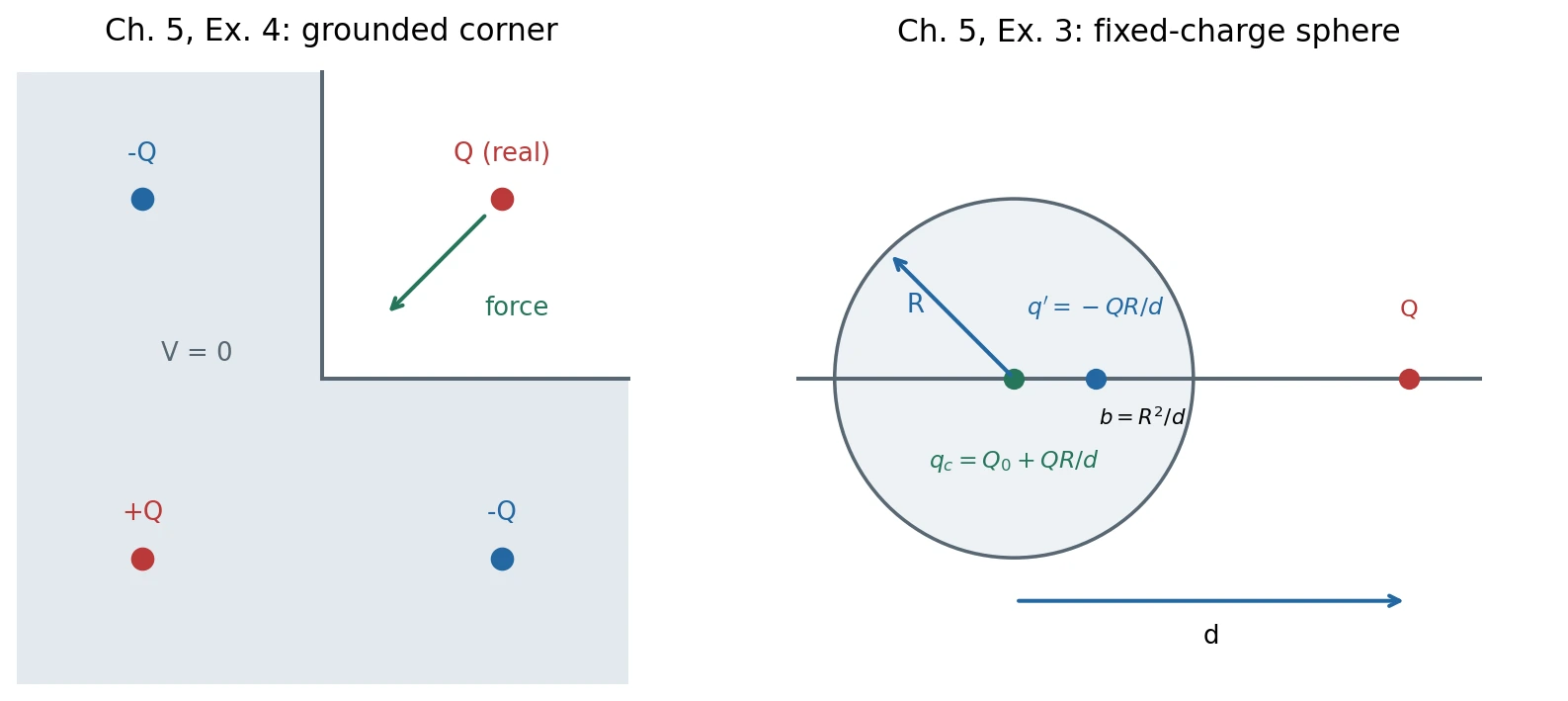
New construction diagrams for chap05.pdf, Ex. 4 (left) and Ex. 3 (right), PDF p. 9 / printed p. 42; figure record.

Ch. 5, Ex. 3 · An isolated charged conducting sphere

Problem. A point charge \(Q\) is outside a thin conducting spherical shell of radius \(R\), at center-distance \(d>R\). The shell is isolated, with total charge \(Q_0\). Find the force on \(Q\).

Method: Spherical image construction, with a fixed-charge condition.

Solution. Let \(\hat{\mathbf n}\) point from the center to \(Q\). The grounded-sphere images are \(q'=-QR/d\) at \(b=R^2/d\) along \(\hat{\mathbf n}\). For the isolated sphere add a central image

\[ q_c=Q_0-q'=Q_0+\frac{QR}{d}. \]

The pair \(Q,q'\) gives zero potential on the sphere; \(q_c\) adds the constant \(kq_c/R\) and makes the represented shell charge \(q'+q_c=Q_0\). Uniqueness then fixes the exterior solution. The force is the force of both images, excluding the real charge's own field:

\[ \boxed{\mathbf F= \left[\frac{kQ(Q_0+QR/d)}{d^2} -\frac{kQ^2Rd}{(d^2-R^2)^2}\right]\hat{\mathbf n}.} \]

For \(Q_0=0\) the net force is attractive. 有净电荷的孤立球需要中心补偿电荷；不能直接套用接地球的单镜像结果。

Ch. 5, Ex. 4 · Two perpendicular grounded walls

Problem. A charge \(Q\) is at \((a,a,0)\), \(a>0\). A grounded conductor fills \(x<0\) or \(y<0\) (including their overlap); the empty region is \(x,y>0\). Find the conductor's force on \(Q\).

Method: Images and uniqueness.

Solution. Use three images:

Image position	Charge	Force on the real charge
\((-a,a,0)\)	\(-Q\)	\(-kQ^2\hat{\mathbf x}/(4a^2)\)
\((a,-a,0)\)	\(-Q\)	\(-kQ^2\hat{\mathbf y}/(4a^2)\)
\((-a,-a,0)\)	\(+Q\)	\(kQ^2(\hat{\mathbf x}+\hat{\mathbf y})/(8\sqrt2a^2)\)

Charges cancel in pairs on each boundary plane, so both planes have \(V=0\). Superposition gives

\[ \boxed{\mathbf F=-\frac{kQ^2}{4a^2} \left(1-\frac1{2\sqrt2}\right)(\hat{\mathbf x}+\hat{\mathbf y}).} \]

It points toward the corner along the bisector, with magnitude \(\sqrt2kQ^2[1-1/(2\sqrt2)]/(4a^2)\). A second negative image alone would spoil the first plane's boundary condition; the positive diagonal image restores both.

Ch. 5, Ex. 8 · Connected spheres and sharp points

Problem. Spheres of radii \(R_1>R_2\) are far apart and joined by a thin wire. They carry total charge \(Q>0\). Set \(V(\infty)=0\), neglect wire charge and mutual influence, and treat each sphere's charge as uniform. (a) Find \(Q_1,Q_2\). (b) Find \(\sigma_1/\sigma_2\), \(E_1/E_2\), and the implication for a conductor's sharp points.

Method: Equipotential conductors and sphere surface fields.

Solution. (a) The connected conductor has one potential:

\[ \frac{kQ_1}{R_1}=\frac{kQ_2}{R_2},\qquad Q_1+Q_2=Q, \qquad \boxed{Q_1=\frac{QR_1}{R_1+R_2},\quad Q_2=\frac{QR_2}{R_1+R_2}.} \]

(b) From \(\sigma_i=Q_i/(4\pi R_i^2)\) and \(E_i=\sigma_i/\epsilon_0\),

\[ \boxed{\frac{\sigma_1}{\sigma_2}=\frac{E_1}{E_2}=\frac{R_2}{R_1}<1.} \]

The smaller sphere has less total charge but a stronger surface field. This illustrates field enhancement near small-radius, sharp regions（尖端效应）; the exact ratio here relies on the widely separated sphere approximation.

Ch. 6, Ex. 5 · Wire above a grounded plane

Problem. A long wire of radius \(a\) runs parallel to an infinite grounded metal plane, with its axis at height \(h\gg a\). The gap is vacuum. Find the capacitance per unit length using a line-charge image.

Method: Plane images and capacitance from \(Q/V\).

Solution. Replace the wire by \(+\lambda\) at height \(h\) and its image by \(-\lambda\) at \(-h\). At a field point whose distances from the two lines are \(r_+,r_-\),

\[ V=\frac{\lambda}{2\pi\epsilon_0}\ln\frac{r_-}{r_+}. \]

The plane has \(r_-=r_+\), hence \(V=0\). On the thin wire, \(r_+\simeq a\) and \(r_-\simeq2h\), giving

\[ V_{\rm wire}\simeq\frac{\lambda}{2\pi\epsilon_0}\ln\frac{2h}{a}, \qquad \boxed{C'=\frac{\lambda}{V_{\rm wire}}\simeq\frac{2\pi\epsilon_0}{\ln(2h/a)}.} \]

\(C'\) has units F/m. The stated \(h\gg a\) makes the geometric-axis line approximation valid. For comparison, placing the exact image lines at heights \(\pm\sqrt{h^2-a^2}\) makes the circular wire an exact equipotential and gives \(C'=2\pi\epsilon_0/\operatorname{arcosh}(h/a)\), with the same thin-wire limit.

Ch. 6, Ex. 7 · Charge at a conductivity interface

Problem. Two long rods, each of area \(S\) and conductivities \(\sigma_1,\sigma_2\), are joined end to end along \(x\). A steady uniform current \(I>0\) flows from rod 1 into rod 2 along \(+x\). Both permittivities are \(\epsilon_0\). (a) Find the fields and explain why they can differ. (b) Find the interface free charge and when it is positive.

Method: Local Ohm's law and normal-field discontinuity.

Solution. (a) Charge conservation fixes the same \(J=I/S\), not the same \(E\):

\[ \boxed{\mathbf E_1=\frac{I}{S\sigma_1}\hat{\mathbf x},\qquad \mathbf E_2=\frac{I}{S\sigma_2}\hat{\mathbf x}.} \]

(b) A thin pillbox across the interface gives \(\sigma_{s}=\epsilon_0(E_2-E_1)\), so

\[ \boxed{Q_{\rm interface}=S\sigma_s =\epsilon_0I\left(\frac1{\sigma_2}-\frac1{\sigma_1}\right).} \]

It is positive for \(\sigma_1>\sigma_2\), zero for equal conductivities, and negative for \(\sigma_1<\sigma_2\). 界面电荷建立所需的电场差，使稳态电流连续。

Ch. 6, Ex. 8 · Hemispherical earth electrode

Problem. A metal hemisphere of radius \(a\) is buried with its flat face at the ground surface. Ground conductivity \(\sigma\) is much smaller than the metal's; air is nonconducting. Steady current \(I\) flows radially out through the ground to a very distant return electrode. Let \(V(\infty)=0\). (a) Find \(\mathbf J,\mathbf E\) for \(r>a\) and the electrode resistance. (b) Find the voltage between feet at \(r\) and \(r+s\) on one radial line; explain the effect of reducing \(s\).

Method: Current density and resistance, using a hemispherical current surface.

Solution. (a) Current crosses area \(2\pi r^2\), so

\[ \boxed{\mathbf J=\frac I{2\pi r^2}\hat{\mathbf r},\qquad \mathbf E=\frac I{2\pi\sigma r^2}\hat{\mathbf r}.} \]

Integrating the field,

\[ V(r)=\int_r^\infty E(s')ds'=\frac I{2\pi\sigma r}, \qquad \boxed{R=\frac{V(a)}I=\frac1{2\pi\sigma a}.} \]

(b) The step voltage（跨步电压）is

\[ \boxed{V(r)-V(r+s)=\frac I{2\pi\sigma}\left(\frac1r-\frac1{r+s}\right) =\frac{Is}{2\pi\sigma r(r+s)}.} \]

At fixed \(r\), reducing foot separation reduces this voltage and the resulting body current in this model. Near the electrode the radial potential gradient is largest.

Ch. 7, Ex. 3 · Wheatstone bridge with source resistance

Problem. In the bridge below, \(r_1\) joins \(A\)–\(C\), \(r_3\) joins \(C\)–\(B\), \(r_2\) joins \(A\)–\(D\), \(r_4\) joins \(D\)–\(B\), and \(r_g\) joins \(C\)–\(D\). The source branch has emf \(\mathcal E\) (positive terminal toward \(B\)) and series resistance \(r_0\). (a) Find \(I\) through \(r_g\), positive from \(C\) to \(D\). (b) Find the zero-current condition.

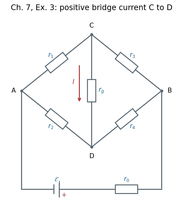
Redrawn from chap07.pdf, Fig. 7.7, PDF p. 9 (printed p. 62); figure record.

Method: Kirchhoff node and loop rules.

Solution. (a) Set \(V_A=0\), \(V_B=V\), \(V_C=u\), \(V_D=w\). The node equations are

\[ \frac u{r_1}+\frac{u-V}{r_3}+\frac{u-w}{r_g}=0, \qquad \frac w{r_2}+\frac{w-V}{r_4}+\frac{w-u}{r_g}=0, \]

\[ \frac{\mathcal E-V}{r_0}=\frac{V-u}{r_3}+\frac{V-w}{r_4}, \qquad I=\frac{u-w}{r_g}. \]

Solving this linear system gives

\[ \boxed{I=\frac{\mathcal E(r_1r_4-r_2r_3)}{r_g\mathcal A+\mathcal B},} \]

where

\[ \begin{aligned} \mathcal A&=(r_1+r_3)(r_2+r_4)+r_0(r_1+r_2+r_3+r_4),\\ \mathcal B&=r_1r_2(r_3+r_4)+r_3r_4(r_1+r_2) +r_0(r_1+r_2)(r_3+r_4). \end{aligned} \]

For an ideal source use the \(r_0\to0\) limit (or set \(V=\mathcal E\) directly).

(b) For positive finite resistances, the denominator is positive; therefore

\[ \boxed{I=0\iff r_1r_4=r_2r_3\iff\frac{r_1}{r_2}=\frac{r_3}{r_4}.} \]

At balance \(V_C=V_D\): the bridge branch draws no current. The balance condition is independent of \(r_0\) and \(r_g\); the current away from balance is not.

Ch. 7, Ex. 5 · Charging with three resistors

Problem. Three branches join nodes \(A,B\): a capacitor \(C\) in series with \(r_3\), a resistor \(r_2\), and a source \(\mathcal E\) (positive toward \(B\)) in series with \(r_1\) and a switch. The capacitor is uncharged when the switch closes at \(t=0\). Find the magnitude \(q(t)\) of either plate's charge and \(q(\infty)\).

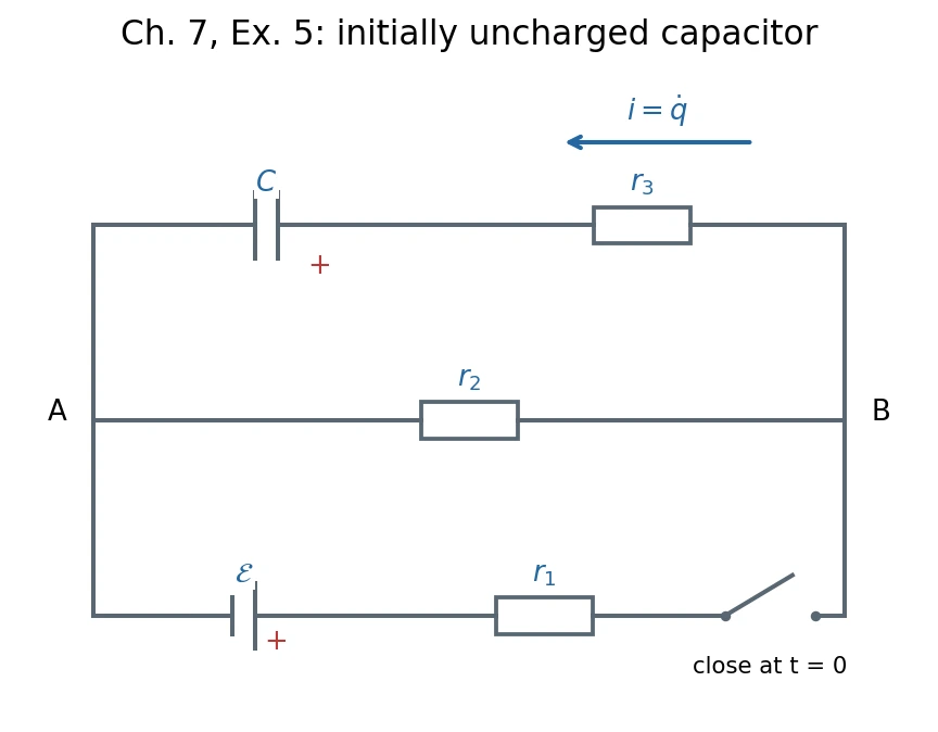
Redrawn from chap07.pdf, Fig. 7.9, PDF p. 10 (printed p. 63); figure record.

Method: Kirchhoff rules and first-order RC response.

Solution. Let \(V=V_B-V_A\), and let \(i=\dot q\) flow from \(B\) through \(r_3\) into the capacitor's positive plate. Then

\[ \frac{\mathcal E-V}{r_1}=\frac V{r_2}+i, \qquad V=r_3i+\frac qC. \]

Eliminating \(V\) gives

\[ R_*\dot q+\frac qC=\mathcal E_*,\qquad R_*=r_3+\frac{r_1r_2}{r_1+r_2},\qquad \mathcal E_*=\frac{r_2}{r_1+r_2}\mathcal E. \]

With \(q(0)=0\),

\[ \boxed{q(t)=C\mathcal E_*\left(1-e^{-t/(CR_*)}\right), \qquad q(\infty)=\frac{C\mathcal E r_2}{r_1+r_2}.} \]

At long times the capacitor branch carries no current and the remaining divider fixes its voltage. 时间常数中的电阻是 \(r_3+(r_1\parallel r_2)\)，不是三个电阻直接相加。

Ch. 7, Ex. 9 · Capacitor force and battery work

Problem. A vacuum parallel-plate capacitor has area \(S\), separation \(x\), a fixed lower plate, and a movable upper plate. Ignore edges and move slowly, neglecting kinetic energy and heat. Force \(F\) is positive toward increasing \(x\). (a) For isolated charges \(\pm q\), find \(U(x)\) and \(F\). (b) With an ideal battery holding voltage \(V\), find \(U(x)\), battery work for \(dx\), and the correct force from energy conservation; explain the failure of simply using \(-dU/dx\) and compare with (a).

Method: Capacitor energy and source power.

Solution. (a) Since \(C=\epsilon_0S/x\) and \(q\) is fixed,

\[ U(x)=\frac{q^2}{2C}=\frac{q^2x}{2\epsilon_0S},\qquad \boxed{F=-\left.\frac{dU}{dx}\right|_q=-\frac{q^2}{2\epsilon_0S}.} \]

(b) At fixed \(V\),

\[ U(x)=\frac12CV^2=\frac{\epsilon_0SV^2}{2x},\qquad q(x)=\frac{\epsilon_0SV}{x},\qquad \delta W_{\rm battery}=V\,dq=-\frac{\epsilon_0SV^2}{x^2}dx. \]

Energy balance is \(dU=\delta W_{\rm battery}-F\,dx\) (the external agent does work \(-F\,dx\)). Hence

\[ \boxed{F=\frac{\delta W_{\rm battery}}{dx}-\frac{dU}{dx} =-\frac{\epsilon_0SV^2}{2x^2}.} \]

Using \(-dU/dx\) alone omits energy returned to the battery and gives the wrong sign. Both answers are attractive and agree at \(q=CV\): \(|F|/S=\epsilon_0E^2/2\). 固定电荷与固定电压的能量系统边界不同，电池做功不能漏掉。